


 Stein损失函数下层次模型正参数的经验贝叶斯估计


目录
笔记
搜索

【点击观看 AI 速读解析视频,轻松读懂全书重点】
Preface
The book aims to develop empirical Bayes estimators for positive parameters in seven hierarchical models under Stein’s loss function, with theoretical derivations, simulations, and real data examples.
Chapter 1 is an introduction, including introductory texts on the empirical Bayes method, gamma and inverse gamma distributions, hierarchical models with positive restricted parameters, estimating the hyperparameters, Stein’s loss function, Bayes estimators and Posterior Expected Stein’s Losses (PESLs), theoretical comparisons of the Bayes estimators and the PESLs of three methods, simulation techniques, and R codes. Chapters 2–8 contain the main results of the research. Each chapter deals with a different hierarchical model, and calculates the empirical Bayes estimators of the positive parameter of the hierarchical model under Stein’s loss function. Chapter 9 is devoted to 16 common loss functions, namely, squared error loss function, weighted squared error loss function, Stein’s loss function, power-power loss function, power-log loss function, Zhang’s loss function, LINEX loss function, absolute error loss function, weighted absolute error loss function, power loss function, weighted power loss function, log-1 loss function, log-2 loss function, generalized log loss function, generalized Stein’s loss function, and generalized power-power loss function. Chapter 10 contains some summaries and discussions of the book. Appendix A contains some technical derivations of the results in chapters 2–8. Appendix B summarizes some basic results on common univariate distributions.
The contents of chapters 2–8 are summarized in table 1. From the table, we observe the following facts.
1. Each chapter contains a theoretical section, simulations section, and/or a real data section.
2. For the theoretical section, every chapter contains two subsections: Bayes estimators and PESLs, and empirical Bayes estimators of  .
.
.
3. For the simulations section, every chapter contains four subsections: Two inequalities of Bayes estimators and PESLs, consistencies of moment estimators and Maximum Likelihood Estimators (MLEs), goodness-of-fit of the model, and marginal distributions for various hyperparameters.
4. If a chapter contains a subsection, then we place a  . However, if a chapter does not contain a subsection, then we place a
  .
.
. However, if a chapter does not contain a subsection, then we place a .
5. The marginal distributions of the first six hierarchical models (Inverse Gamma-Inverse Gamma (IG-IG), Gamma-Gamma (G-G), Exponential-Inverse Gamma (Exp-IG), Normal-Inverse Gamma (N-IG), Normal-Normal Inverse Gamma (N-NIG), and Uniform-Inverse Gamma (U-IG)) are continuous. Thus they can be used to model continuous data. The Kolmogorov-Smirnov (KS) test is used to perform the goodness-of-fit of the model to the data. The marginal distribution of the last hierarchical model (Poisson-Gamma (P-G)) is discrete, and thus it can be used to model discrete data. The chi-square test is utilized to perform the goodness-of-fit of the model to the data.
TAB. 1 — P: The contents of chapters 2–8.
| Subsection | IG-IG | G-G | Exp-IG | N-IG | N-NIG | U-IG | P-G | |
| Theoretical section | Bayes estimators and PESLs |  |
 |
 |
 |
 |
 |
 |
Empirical Bayes estimators of  |
 |
 |
 |
 |
 |
 |
 |
|
| Theoretical comparisons of Bayes estimators and PESLs of three methods |  |
 |
 |
 |
 |
 |
 |
|
| Simulations section | Two inequalities of Bayes estimators and PESLs |  |
 |
 |
 |
 |
 |
 |
| Consistencies of moment estimators and MLEs |  |
 |
 |
 |
 |
 |
 |
|
| Goodness-of-fit of the model |  |
 |
 |
 |
 |
 |
 |
|
| Numerical comparisons of Bayes estimators and PESLs of three methods |  |
 |
 |
 |
 |
 |
 |
|
| Marginal distributions for various hyperparameters |  |
 |
 |
 |
 |
 |
 |
|
| Real data section | A real data example |  |
 |
 |
 |
 |
 |
 |
In the Table of Contents, List of Figures, List of Tables, List of Abbreviations, and appendix A, there are some abbreviations. They are used to indicate relevant chapters. More specifically, IG-IG, G-G, Exp-IG, N-IG, N-NIG, U-IG, and P-G are used to indicate relevant chapters of hierarchical models. P is short for Preface. LoA is short for List of Abbreviations. I is short for Introduction. SCLF is short for Several Common Loss Functions.
This book is supported by the First Class Construction Fund for Statistics Discipline of Yunnan University and the High-level Talent Research Start-up Fund Project of Yunnan University.
Ying-Ying Zhang
October, 2025
Chapter 1 Introduction
1.1 Empirical Bayes Method
In this section, we will introduce some literature on the empirical Bayes method, statistical inference, and Bayesian books.
The empirical Bayes method relies on a conjugate prior modeling, where the hyperparameters are estimated from the observations, and the “estimated prior” is then used as a regular prior in the subsequent inference. See Carlin and Louis (2000a); Maritz and Lwin (1989); Berger (1985) and the references therein. The empirical Bayes method is introduced in Robbins (1955, 1964, 1983). From a Bayesian point of view, it means that the sampling distribution is known, but the prior distribution is not. The marginal distribution is then used to recover the prior distribution from the observations. More literature on empirical Bayes method can be found, for example, in Li et al. (2025); Shi et al. (2025); Zhang (2025); Sun et al. (2024); Zhang et al. (2024); Sun et al. (2021); Zhou et al. (2021); Mikulich-Gilbertson et al. (2019); Zhang et al. (2019a, 2019b); Martin et al. (2017); Satagopan et al. (2016); Ghosh et al. (2015); van Houwelingen (2014); Efron (2011); Coram and Tang (2007); Pensky (2002); Carlin and Louis (2000b); Maritz and Lwin (1992); Morris (1983); Deely and Lindley (1981).
Statistical inferences are covered by many classical textbooks, see for instance, Shi and Tao (2008); Lehmann and Romano (2005); Shao (2003); Casella and Berger (2002); Stuart et al. (1999); Lehmann and Casella (1998); Bickel and Doksum (1977); Ferguson (1967). Point estimation is an important class of statistical inference. The study of the performance and the optimality of point estimators is usually evaluated through the loss function. In Bayesian analysis, we usually compute the Bayes risk to assess the performance of an estimator with respect to a given loss function.
Bayesian approaches are continually developing, and some of the most important works are Huang (2021); Wei and Zhang (2021); Wu (2021); Jiang (2020); Wu (2020); Han (2017); Huang (2017a, 2017b); Liu and Xia (2016); Wei (2016); Han (2015); Wei (2015); Gelman et al. (2013); Lee (2011); Albert (2009); Robert and Casella (2009); Robert (2007); Robert and Casella (2005); Chen et al. (2000); Bernardo and Smith (1994); Box and Tiao (1992); Berger (1985); Novick and Jackson (1974); Savage (1972); Zellner (1971); DeGroot (1970); Good (1965); Lindley (1965).
1.2 The Gamma and Inverse Gamma Distributions
In this section, we will give the probability density functions (pdfs) of the gamma and inverse gamma distributions.
Suppose that  and
and  . More specifically, the pdfs of
  and
and  are respectively given by

and . More specifically, the pdfs of and are respectively given by
It is easy to calculate
 and
and

Suppose that  and
and  . The pdfs of
  and
and  are respectively given by

and . The pdfs of and are respectively given by
It is easy to calculate
 and
and

For more results about the gamma and inverse gamma distributions, we refer readers to Zhang and Zhang (2022). Positive, continuous, and right-skewed data are fitted by a mixture of gamma and inverse gamma distributions. For 16 hierarchical models of gamma and inverse gamma distributions, there are only 8 of them that have conjugate priors. They first discuss some common typical problems for the 8 hierarchical models that do not have conjugate priors. Then they calculate Bayesian posterior densities and marginal densities of the 8 hierarchical models that have conjugate priors. After that, they discuss relations among the 8 analytical marginal densities. Furthermore, they find some relations among the random variables of the marginal densities and the beta densities. Moreover, they discuss random variable generations for the gamma and inverse gamma distributions by using the R software. In addition, some numerical simulations are performed to illustrate four aspects: the plots of marginal densities, the generations of random variables from the marginal density, the transformations of moment estimators of hyperparameters of a hierarchical model, and the conclusions about the properties of the 8 marginal densities that do not have a closed form. Finally, they have illustrated their method by a real data example, in which the original and transformed data are fitted by the marginal density with different hyperparameters.
1.3 Hierarchical Models with Positive Parameters
In this section, we will introduce 7 hierarchical models with positive parameters. The hierarchical models are in the following general form:
 (1.1)
where
(1.1)
where  are hyperparameters to be estimated,
  ,
,  , or
, or  in this book,
  is the unknown parameter of interest,
  is the distribution of
  with parameter
  , and
, and  is the prior distribution of
  with hyperparameters
  . It is useful to point out that some hyperparameters may exist in
  , and thus
  is more accurate. However, for simplicity, we will use
  . The hierarchical
  models that we will consider in this book are IG-IG (2.1), G-G (3.1), Exp-IG (4.1), N-IG (5.1), N-NIG (6.2), U-IG (7.1), and P-G (8.1).
(1.1)
are hyperparameters to be estimated, , , or in this book, is the unknown parameter of interest, is the distribution of with parameter , and is the prior distribution of with hyperparameters . It is useful to point out that some hyperparameters may exist in , and thus is more accurate. However, for simplicity, we will use . The hierarchical models that we will consider in this book are IG-IG (2.1), G-G (3.1), Exp-IG (4.1), N-IG (5.1), N-NIG (6.2), U-IG (7.1), and P-G (8.1).
1.4 Estimating the Hyperparameters
In this section, we will introduce how to estimate the hyperparameters of the hierarchical model (1.1).
In empirical Bayes analysis, the hyperparameters are unknown, and the marginal distribution is used to estimate the hyperparameters from the observations. There are two common methods to estimate the hyperparameters by exploiting the marginal distribution: the moment method and the Maximum Likelihood Estimation (MLE) method. In this book, we will use the two methods to estimate the hyperparameters of the hierarchical model (1.1).
The moment method to estimate the hyperparameters is performed by equating the population moments to the sample moments. In general, if there are 
 hyperparameters, then we need to calculate the first
  origin moments of
  ,
,  . We can use the iterated expectation method to calculate
  , that is,
 where
where  . Assume that
  can be calculated. Then
 and this expectation may be calculated by noting
  .
.
hyperparameters, then we need to calculate the first origin moments of , . We can use the iterated expectation method to calculate , that is,
. Assume that can be calculated. Then
.
The MLE method to estimate the hyperparameters proceeds as follows. First, we calculate the likelihood function of  :
:
 (1.2)
where
(1.2)
where
 is the marginal distribution of the hierarchical model (1.1),
  is the probability density function (pdf) or probability mass function (pmf) of
  , and
, and  is the prior pdf of
  . Second, we obtain the log-likelihood function of
  :
:

:
(1.2)
is the probability density function (pdf) or probability mass function (pmf) of , and is the prior pdf of . Second, we obtain the log-likelihood function of :
Third, taking partial derivatives with respect to  and setting them to zeros, we obtain

and setting them to zeros, we obtain
Fourth, after some algebra, the above equations reduce to
 (1.3)
(1.3)
 (1.4)
(1.4)

 (1.5)
(1.5)
(1.3)
(1.4)
(1.5)
In general, the analytical calculations of the Maximum Likelihood Estimators (MLEs) of  by solving the equations (1.3), (1.4), ..., and (1.5) are impossible, and thus we have to resort to numerical solutions. Finally, we can exploit Newton’s method to solve the equations (1.3), (1.4), ..., and (1.5) and to numerically obtain the MLEs of
  . The iterative scheme of Newton’s method is
 where
where  is the Jacobian matrix of
  , and
, and  . Note that the MLEs of
  are very sensitive to the initial estimators, and the moment estimators are usually proved to be good initial estimators. The Jacobian matrix can be calculated as follows:
 where
where

by solving the equations (1.3), (1.4), ..., and (1.5) are impossible, and thus we have to resort to numerical solutions. Finally, we can exploit Newton’s method to solve the equations (1.3), (1.4), ..., and (1.5) and to numerically obtain the MLEs of . The iterative scheme of Newton’s method is
is the Jacobian matrix of , and . Note that the MLEs of are very sensitive to the initial estimators, and the moment estimators are usually proved to be good initial estimators. The Jacobian matrix can be calculated as follows:
It is important to note that in calculating (1.2), we have implicitly used the property of independency of  . And this independency property is guaranteed by
 (1.6)
(1.6)
. And this independency property is guaranteed by
(1.6)
If (1.6) is true, then we have
 that is,
 (1.7)
(1.7)
(1.7)
Moreover, if (1.7) is true, then we have (1.6) is true. In other words, (1.6) and (1.7) are equivalent. In addition, (1.7) implies
 (1.8)
(1.8)
(1.8)
It is also important to note that
 (1.9)
can not guarantee (1.8), and vice versa.
(1.9)
can not guarantee (1.8), and vice versa.
(1.9)
1.5 Stein’s Loss Function
In this section, we will introduce Stein’s loss function and justify why Stein’s loss function is better than the squared error loss function on  .
.
.
The (weighted) squared error loss function has been used by many authors for the problem of estimating the variance,  , based on a random sample from a normal distribution with an unknown mean (see, for example, Maatta and Casella (1990); Stein (1964)). As pointed out by Casella and Berger (2002), the (weighted) squared error loss function penalizes equally for overestimation and underestimation, and it is fine for the unrestricted parameter space
  . In the positive parameter space
  where 0 is a natural lower bound, and the estimation problem is not symmetric, we should not select the (weighted) squared error loss function, but select a loss function which penalizes gross overestimation and gross underestimation equally, that is, an action
  will incur an infinite loss when it tends to 0 or ∞. Stein’s loss function has this property, and hence it is recommended to use for the positive parameter space by many authors (see for instance Li et al. (2025); Shi et al. (2025); Zhang (2025); Sun et al. (2024); Zhang et al. (2024); Sun et al. (2021); Bobotas and Kourouklis (2010); Zhang et al. (2019b); Xie et al. (2018); Zhang et al. (2018); Zhang (2017); Oono and Shinozaki (2006); Petropoulos and Kourouklis (2005); Parsian and Nematollahi (1996); Brown (1990, 1968); James and Stein (1961)).
, based on a random sample from a normal distribution with an unknown mean (see, for example, Maatta and Casella (1990); Stein (1964)). As pointed out by Casella and Berger (2002), the (weighted) squared error loss function penalizes equally for overestimation and underestimation, and it is fine for the unrestricted parameter space . In the positive parameter space where 0 is a natural lower bound, and the estimation problem is not symmetric, we should not select the (weighted) squared error loss function, but select a loss function which penalizes gross overestimation and gross underestimation equally, that is, an action will incur an infinite loss when it tends to 0 or ∞. Stein’s loss function has this property, and hence it is recommended to use for the positive parameter space by many authors (see for instance Li et al. (2025); Shi et al. (2025); Zhang (2025); Sun et al. (2024); Zhang et al. (2024); Sun et al. (2021); Bobotas and Kourouklis (2010); Zhang et al. (2019b); Xie et al. (2018); Zhang et al. (2018); Zhang (2017); Oono and Shinozaki (2006); Petropoulos and Kourouklis (2005); Parsian and Nematollahi (1996); Brown (1990, 1968); James and Stein (1961)).
Now, let us give the justifications of why Stein’s loss function is better than the squared error loss function on  . Stein’s loss function is given by
 (1.10)
while the squared error loss function is given by
(1.10)
while the squared error loss function is given by
 (1.11)
. Stein’s loss function is given by
(1.10)
(1.11)
Note that on the positive parameter space  , Stein’s loss function penalizes gross overestimation and gross underestimation equally, that is, an action
  will incur an infinite loss when it tends to 0 or ∞. However, the squared error loss function does not penalize gross overestimation and gross underestimation equally, as an action
  will incur a finite loss (in fact
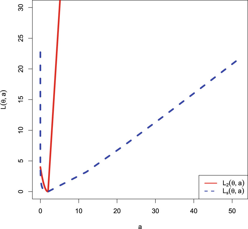
  ) when it tends to 0 and incur an infinite loss when it tends to ∞. Figure 1.1 shows Stein’s loss function and the squared error loss function on
  when
when  .
.
, Stein’s loss function penalizes gross overestimation and gross underestimation equally, that is, an action will incur an infinite loss when it tends to 0 or ∞. However, the squared error loss function does not penalize gross overestimation and gross underestimation equally, as an action will incur a finite loss (in fact ) when it tends to 0 and incur an infinite loss when it tends to ∞. Figure 1.1 shows Stein’s loss function and the squared error loss function on when .
FIG. 1.1 — I: Stein’s loss function and the squared error loss function on  when
when  .
.
when .
For more details of the squared error loss function, the weighted squared error loss function, and Stein’s loss function, we refer readers to relevant subsections in chapter 9.
1.6 The Bayes Estimators and the PESLs
In this section, we will calculate the Bayes estimator of  under Stein’s loss function
  , the Bayes estimator of
  under the usual squared error loss function
  , and the Posterior Expected Stein’s Losses (PESLs) at
  and
and  (
( and
and  ) for any hierarchical model such that the posterior expectations exist.
under Stein’s loss function , the Bayes estimator of under the usual squared error loss function , and the Posterior Expected Stein’s Losses (PESLs) at and ( and ) for any hierarchical model such that the posterior expectations exist.
Similar to Zhang (2017), the two Bayes estimators and the two PESLs are respectively given by
 (1.12)
 (1.13)
 (1.14)
 (1.15)
(1.12)
(1.13)
(1.14)
(1.15)
To calculate the two Bayes estimators and the two PESLs, it remains to calculate

It has been shown in Zhang (2017) that
 (1.16)
by exploiting Jensen’s inequality. Moreover,
(1.16)
by exploiting Jensen’s inequality. Moreover,
 (1.17)
which is a direct consequence of the general methodology for finding a Bayes estimator. According to construction,
(1.17)
which is a direct consequence of the general methodology for finding a Bayes estimator. According to construction,  minimizes the Posterior Expected Stein’s Loss (PESL). In the simulations section and the real data section, we will exemplify the two inequalities (1.16) and (1.17).
(1.16)
(1.17)
minimizes the Posterior Expected Stein’s Loss (PESL). In the simulations section and the real data section, we will exemplify the two inequalities (1.16) and (1.17).
1.7 Theoretical Comparisons of the Bayes Estimators and the PESLs of Three Methods
In this section, similar to Sun et al. (2021), we will theoretically compare the Bayes estimators and the PESLs of the three methods (the oracle method, the moment method, and the MLE method).
Note that the subscripts 0, 1, and 2 below are for the oracle method, the moment method, and the MLE method, respectively. Similar to the derivations in Sun et al. (2021); Zhang (2017), the PESL functions of the three methods are respectively given by
 for
for  .
.
.
Now we calculate the Bayes estimators  and
and  , and the PESLs
  and
and 
 following the route of Sun et al. (2021); Zhang (2017). The Bayes estimators of
  under Stein’s loss function,
 , minimize the corresponding PESL, that is,
 where
where  is the action space,
  is an action (estimator),
  given by (1.10) is Stein’s loss function, and
  is the unknown parameter of interest. Similar to Sun et al. (2021); Zhang (2017), it is easy to obtain
 (1.18)
and , and the PESLs and following the route of Sun et al. (2021); Zhang (2017). The Bayes estimators of under Stein’s loss function, , minimize the corresponding PESL, that is,
is the action space, is an action (estimator), given by (1.10) is Stein’s loss function, and is the unknown parameter of interest. Similar to Sun et al. (2021); Zhang (2017), it is easy to obtain
(1.18)
The Bayes estimators of  under the squared error loss function are given by
 (1.19)
under the squared error loss function are given by
(1.19)
The PESLs evaluated at the Bayes estimators 
 are given by
 (1.20)
are given by
(1.20)
The PESLs evaluated at the Bayes estimators 
 are given by
 (1.21)
are given by
(1.21)
Similar to Sun et al. (2021), our primary objectives are to estimate the Bayes estimators and the PESLs
 by the oracle method. However, the hyperparameters are unknown. The oracle method knows the hyperparameters only in simulations. But in reality, the hyperparameters are unknown.
The good news is that we can actually obtain the Bayes estimators and the PESLs
 by the moment method, and
 by the MLE method, once the data
  are given.
are given.
To compare the moment method and the MLE method, we can compare the Bayes estimators and the PESLs by the two methods with those quantities by the oracle method in simulations. The method that produces closer Bayes estimators and PESLs to the ones by the oracle method in simulations, is a better method.
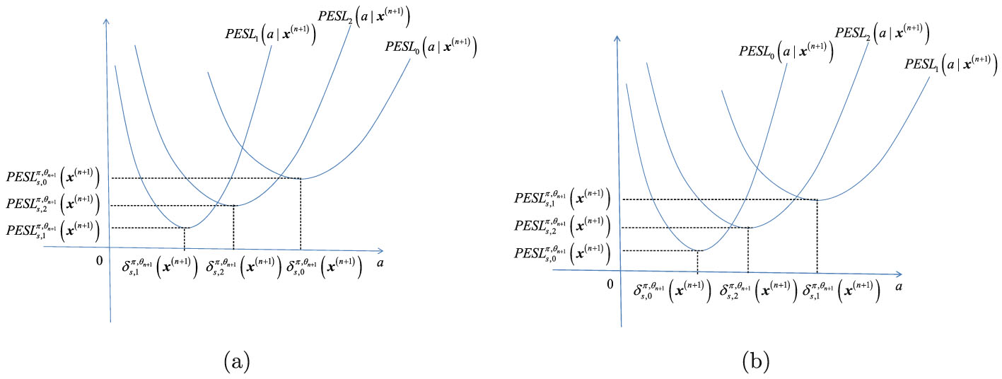
Similar to Sun et al. (2021), the Bayes estimators 
 , the PESL functions
  , and the PESLs
 are depicted in figure 1.2. From the figure, we see that the Bayes estimators
 are the minimizers of the PESL functions
  , and the PESLs
 are the PESL functions
  evaluated at the Bayes estimators
  . Note that for the Bayes estimators,
  and
and  maybe larger or smaller than
  . Similarly, for the PESLs,
  and
and  maybe larger or smaller than
  .
.
, the PESL functions , and the PESLs are depicted in figure 1.2. From the figure, we see that the Bayes estimators are the minimizers of the PESL functions , and the PESLs are the PESL functions evaluated at the Bayes estimators . Note that for the Bayes estimators, and maybe larger or smaller than . Similarly, for the PESLs, and maybe larger or smaller than .
FIG. 1.2 — I: The Bayes estimators  , the PESL functions
  , and the PESLs
  . (a) The Bayes estimators and the PESLs by the oracle method are larger. (b) The Bayes estimators and the PESLs by the oracle method are smaller.
, the PESL functions , and the PESLs . (a) The Bayes estimators and the PESLs by the oracle method are larger. (b) The Bayes estimators and the PESLs by the oracle method are smaller.
1.8 Simulation Techniques
1.8.1 Consistencies of the Moment Estimators and the MLEs
In this subsection, taking the hyperparameters from Sun et al. (2021) as an example, we will introduce a simulation technique to numerically exemplify that the moment estimators ( ,
,  , and
, and  ) and the MLEs (
 ,
,  , and
, and  ) are consistent estimators of the hyperparameters (
 ,
,  , and
, and  ) of the hierarchical inverse gamma and inverse gamma model (2.1). Note that only
  are used in this subsection.
, , and ) and the MLEs (, , and ) are consistent estimators of the hyperparameters (, , and ) of the hierarchical inverse gamma and inverse gamma model (2.1). Note that only are used in this subsection.
Let  denote the hyperparameter
  ,
,  , or
, or  . Then the consistency means that
 for
for  , where
  is for the moment estimator,
  is for the MLE,
  means convergence in probability, and
  is the sample size. Alternatively, the consistency means that
 (1.22)
for every
(1.22)
for every  and every
  . The probabilities are approximated by the corresponding frequencies:
 for
for  , where
  is the indicator function of
  , which is equal to 1 if
  is true and
  otherwise, and
  is the number of simulations. Therefore, the frequencies (
 ,
,  ,
,  , or
, or  ,
,  ) tend to
  means that the estimators are consistent.
denote the hyperparameter , , or . Then the consistency means that
, where is for the moment estimator, is for the MLE, means convergence in probability, and is the sample size. Alternatively, the consistency means that
(1.22)
and every . The probabilities are approximated by the corresponding frequencies:
, where is the indicator function of , which is equal to 1 if is true and otherwise, and is the number of simulations. Therefore, the frequencies (, , , or , ) tend to means that the estimators are consistent.
1.8.2 Goodness-of-Fit of the Model
In this subsection, we will introduce two simulation techniques to calculate the goodness-of-fit of the hierarchical model to the simulated data (see Ross (2013); Xue and Chen (2007)). The first simulation technique is the chi-square test, which is mainly used for discrete distributions. The second simulation technique is the Kolmogorov-Smirnov (KS) test, which is mainly used for continuous distributions. Note that only  are used in this subsection.
are used in this subsection.
Chi-square test
Let us take the hierarchical Poisson and gamma model (8.1) as an example to illustrate the process of the chi-square test. Two cases of the goodness-of-fit will be considered. In the first case, the hyperparameters  and
and  are assumed known. In the second case, the hyperparameters
  and
and  are unknown, and this is also the case encountered in real applications.
and are assumed known. In the second case, the hyperparameters and are unknown, and this is also the case encountered in real applications.
Case 1. The hyperparameters  and
and  are assumed known.
and are assumed known.
In this case, the hyperparameters  and
and  are assumed known. For example,
  and
and  . Let the null hypothesis be
 where
where  is the marginal distribution of the hierarchical Poisson and gamma model (8.1) with the marginal pmf
  given by (8.3).
and are assumed known. For example, and . Let the null hypothesis be
is the marginal distribution of the hierarchical Poisson and gamma model (8.1) with the marginal pmf given by (8.3).
The chi-square goodness-of-fit is performed as follows. We first divide the domain of  ,
,  , into
  groups:

, , into groups:
Let the theoretical probabilities under  on these subintervals be
 where
where

 and
and  is the probability when
  is distributed under
  . Let
. Let  , denote the number of
  that lie in the
  th subinterval
  . Then the chi-square statistics (Ross (2013); Xue and Chen (2007))
 where
where  is convergence in distribution. Moreover, we can compute the p-value, which gives the probability that a value of
  as large as
  would have occurred if the null hypothesis were true. Hence,
 where pchisq(), which calculates the cumulative distribution function (cdf) of a chi-square random variable, is an R built-in function (R Core Team (2023)). Note that a large p-value (>0.05 in the usual case) indicates that the model specified by
  fits the (simulated) data well, while a small p-value (≤0.05 in the usual case) indicates that the model specified by
  does not fit the (simulated) data well. The larger the p-value, the better the model specified by
  fits the (simulated) data.
on these subintervals be
is the probability when is distributed under . Let , denote the number of that lie in the th subinterval . Then the chi-square statistics (Ross (2013); Xue and Chen (2007))
is convergence in distribution. Moreover, we can compute the p-value, which gives the probability that a value of as large as would have occurred if the null hypothesis were true. Hence,
fits the (simulated) data well, while a small p-value (≤0.05 in the usual case) indicates that the model specified by does not fit the (simulated) data well. The larger the p-value, the better the model specified by fits the (simulated) data.
Case 2. The hyperparameters  and
and  are unknown.
and are unknown.
Let the null hypothesis be
 where
where  and
and  are unknown. First, the hyperparameters
  and
and  need to be estimated by the sample. The estimators could be the moment estimators or the MLEs. Let
  and
and  be given in Case 1. The theoretical probabilities under
  on the subintervals are calculated by
 that is, the unknown hyperparameters
  and
and  are estimated by their estimators
  and
and  based on the sample. Then the chi-square statistics (Ross (2013); Xue and Chen (2007))

and are unknown. First, the hyperparameters and need to be estimated by the sample. The estimators could be the moment estimators or the MLEs. Let and be given in Case 1. The theoretical probabilities under on the subintervals are calculated by
and are estimated by their estimators and based on the sample. Then the chi-square statistics (Ross (2013); Xue and Chen (2007))
Note that the degree of freedom is now lost by 2, since two unknown parameters are estimated by the sample. Moreover, the p-value is given by

KS test
Chi-square test is a measure of the goodness-of-fit. However, the chi-square test is very sensitive because of the problem of choosing the number of groups and the problem of finding the cut-points. Therefore, instead of using the chi-square test as a measure of the goodness-of-fit, we may use the Kolmogorov-Smirnov test (or the KS test) as a measure of the goodness-of-fit.
The Kolmogorov-Smirnov statistic is the distance  between the empirical cdf
  and the population cdf
  , that is,
 (1.23)
between the empirical cdf and the population cdf , that is,
(1.23)
In R software, the built-in function ks.test() can perform the KS test (see Marsaglia et al. (2003); Durbin (1973); Conover (1971)). Note that the KS test is generally valid for one-dimensional continuous cumulative distribution functions (cdfs). But in literature, KS-type tests have been developed for discrete data too (Santitissadeekorn et al. (2020); Aldirawi et al. (2019); Dimitrova et al. (2020)).
The return value of ks.test() is a list containing the components statistic (the value of the test statistic, or the  value) and p-value (the p-value of the test). It is well known in the literature that a smaller
  value or a larger p-value indicates a better fit of the model to the simulated data. Inspired by and based on the
  value and p-value, Sun et al. (2021) propose five indices (
 ,
,  ,
,  ,
,  , and
, and  ) to compare the three methods, namely, the oracle method, the moment method, and the MLE method in simulations.
  is the average
  values (1.23) of
  simulations (the smaller the better).
  is the average p-value of
  simulations (the larger the better).
  is the percentage of
  simulations that attain the minimum
  value in the three methods (the larger the better). The three
  values should sum to
  .
.  is the percentage of
  simulations which attain the maximum p-value in the three methods (the larger the better). The three
  values should sum to
  .
.  is the percentage of accepting
  (defined as p-value >0.05) in
  simulations for each method (the larger the better). Each
  value should between 0%–100%.
value) and p-value (the p-value of the test). It is well known in the literature that a smaller value or a larger p-value indicates a better fit of the model to the simulated data. Inspired by and based on the value and p-value, Sun et al. (2021) propose five indices (, , , , and ) to compare the three methods, namely, the oracle method, the moment method, and the MLE method in simulations. is the average values (1.23) of simulations (the smaller the better). is the average p-value of simulations (the larger the better). is the percentage of simulations that attain the minimum value in the three methods (the larger the better). The three values should sum to . is the percentage of simulations which attain the maximum p-value in the three methods (the larger the better). The three values should sum to . is the percentage of accepting (defined as p-value >0.05) in simulations for each method (the larger the better). Each value should between 0%–100%.
1.8.3 Numerical Comparisons of the Bayes Estimators and the PESLs of Three Methods
In this subsection, we will introduce two simulation techniques to numerically compare the Bayes estimators and the PESLs of the three methods (the oracle method, the moment method, and the MLE method). The first simulation technique is to calculate the averages and proportions of the absolute errors from the oracle method by the moment method and the MLE method, for the estimators of the hyperparameters, the Bayes estimators, and the PESLs. The second simulation technique is to calculate the Mean Square Error (MSE), Mean Absolute Error (MAE), and Mean Entropy Error (MEE) of the estimators of the hyperparameters.
The averages and proportions of the absolute errors
We can calculate the averages and proportions of the absolute errors from the oracle method by the moment method and the MLE method for the estimators of the hyperparameters, the Bayes estimators, and the PESLs. The averages of the absolute errors from the oracle method by the moment method and the MLE method are the sample averages of the absolute error vectors from the oracle method by the moment method and the MLE method; the smaller the better. The proportions of the absolute errors from the oracle method, by the moment method, and the MLE method are the sample proportions of the absolute errors by the method being equal to the minimum of the two absolute errors, the larger the better.
We will only give the mathematical formulas of the averages and proportions of the absolute errors from the oracle method by the moment method and the MLE method for the Bayes estimator under Stein’s loss function  . These quantities for the estimators of the hyperparameters, the Bayes estimator
  , and the PESLs
  and
and  are similar, and thus they are omitted.
. These quantities for the estimators of the hyperparameters, the Bayes estimator , and the PESLs and are similar, and thus they are omitted.
To calculate the averages and proportions of the absolute errors from the oracle method by the moment method, and the MLE method for  , we need the absolute error vectors by the moment method and the MLE method for
  , which are respectively given by
 and
and

, we need the absolute error vectors by the moment method and the MLE method for , which are respectively given by
The averages of the absolute errors from the oracle method by the moment method, and the MLE method for  are the sample averages of the absolute error vectors
  and
and  , and the averages are respectively given by
 and
and

are the sample averages of the absolute error vectors and , and the averages are respectively given by
With the two absolute error vectors  and
and  , we can compute a parallel minima vector of the absolute error vectors by
 where pmin() is an R built-in function which returns a single vector giving the parallel minima of the argument vectors. Finally, the proportions
  and
and  of the absolute errors from the oracle method by the moment method, and the MLE method for
  are computed by
 and
and
 where
where  is the indicator function of
  which is equal to
  if
if  is true and
  otherwise. To avoid the case of equal absolute errors from the oracle method by the moment method, and the MLE method for
  , we could compute
 to ensure that the two proportions sum to
  .
.
and , we can compute a parallel minima vector of the absolute error vectors by
and of the absolute errors from the oracle method by the moment method, and the MLE method for are computed by
is the indicator function of which is equal to if is true and otherwise. To avoid the case of equal absolute errors from the oracle method by the moment method, and the MLE method for , we could compute
.
MSE, MAE, and MEE
The MSE, MAE, and MEE are criteria to compare two different estimators. The MSE, MAE, and MEE are risk functions (expected loss functions) of the estimators of the hyperparameters, and they could measure the performance of the estimators. The smaller the MSE, MAE, and MEE values, the better the estimator.
Let  be a hyperparameter. Let
  be an estimator of θ, where
  is for the moment estimator and
  is for the MLE. The MSE of the estimator
  is defined by (see Casella and Berger (2002))

be a hyperparameter. Let be an estimator of θ, where is for the moment estimator and is for the MLE. The MSE of the estimator is defined by (see Casella and Berger (2002))
Similarly, the MAE of the estimator  is defined by (see Casella and Berger (2002))

is defined by (see Casella and Berger (2002))
Moreover, the MEE of the estimator  is defined by
 where the entropy loss function is also known as Stein’s loss function, given by (1.10).
is defined by
1.9 R Codes
The R codes for the hierarchical IG-IG, G-G, Exp-IG, N-IG, N-NIG, U-IG, and P-G models and the figures of Several Common Loss Functions are available at Édition Diffusion Press (EDP) Sciences bookshop website: https://laboutique.edpsciences.fr/produit/1511/9782759839124/empirical-bayes-estimators-of-positive-parameters-in-hierarchical-models-under-stein-s-loss-function. Alternatively, one can send an email to the author at robertzhangyying@qq.com.
Chapter 2 The Empirical Bayes Estimators of the Rate Parameter of the Inverse Gamma Distribution with a Conjugate Inverse Gamma Prior under Stein’s Loss Function
For the hierarchical inverse gamma and inverse gamma model, we calculate the Bayes estimator of the rate parameter of the inverse gamma distribution under Stein’s loss function, which penalizes gross overestimation and gross underestimation equally, and the corresponding PESL. We also obtain the Bayes estimator of the rate parameter under the squared error loss and the corresponding PESL. Moreover, we obtain the empirical Bayes estimators of the rate parameter of the inverse gamma distribution with a conjugate inverse gamma prior by the moment and MLE methods under Stein’s loss function. In numerical simulations, we have illustrated five aspects: The two inequalities of the Bayes estimators and the PESLs for the oracle method; the moment estimators and the MLEs are consistent estimators of the hyperparameters; the goodness-of-fit of the model to the simulated data; the comparisons of the Bayes estimators and the PESLs of the oracle, moment, and MLE methods; and the marginal densities of the model for various hyperparameters. The numerical results indicate that the MLEs are better than the moment estimators when estimating the hyperparameters. Finally, the model could potentially be used to fit right-skewed data, not left-skewed data.
Acknowledgement. This chapter is derived in part from an article Sun et al. (2021) published in the Journal of Statistical Computation and Simulation, 12 December 2020 <copyright Taylor & Francis>, available online: http://www.tandfonline.com/10.1080/00949655.2020.1858299.
2.1 Introduction
Since the rate parameter of the inverse gamma distribution with a conjugate inverse gamma prior is a positive parameter,  , the Bayes estimator of
  under the squared error loss function, is not appropriate. In contrast, we should select Stein’s loss function because it penalizes gross overestimation and gross underestimation equally. To determine the unknown hyperparameters, we adopt the empirical Bayes method. In this chapter, we calculate the Bayes estimator of
  under Stein’s loss function and the corresponding PESL. We also obtain the Bayes estimator of
  under the squared error loss function and the corresponding PESL. Moreover, we obtain the empirical Bayes estimators of the rate parameter
  of the inverse gamma distribution with a conjugate inverse gamma prior by the moment method and the MLE method under Stein’s loss function.
, the Bayes estimator of under the squared error loss function, is not appropriate. In contrast, we should select Stein’s loss function because it penalizes gross overestimation and gross underestimation equally. To determine the unknown hyperparameters, we adopt the empirical Bayes method. In this chapter, we calculate the Bayes estimator of under Stein’s loss function and the corresponding PESL. We also obtain the Bayes estimator of under the squared error loss function and the corresponding PESL. Moreover, we obtain the empirical Bayes estimators of the rate parameter of the inverse gamma distribution with a conjugate inverse gamma prior by the moment method and the MLE method under Stein’s loss function.
The rest of the chapter is organized as follows. In section 2.2, we calculate the Bayes estimators and the PESLs, and they satisfy two inequalities (2.6) and (2.9). Moreover, we summarize the empirical Bayes estimators of the parameter of the model (2.1) under Stein’s loss function by the moment method and the MLE method in Theorem 2.4. Furthermore, we have theoretically compared the Bayes estimators and the PESLs of the three methods (the oracle method, the moment method, and the MLE method). In section 2.3, we will carry out some numerical simulations, where we will illustrate five aspects. First, we will numerically exemplify the two inequalities of the Bayes estimators and the PESLs for the oracle method. Second, we will illustrate that the moment estimators and the MLEs are consistent estimators of the hyperparameters. Third, we will calculate the goodness-of-fit of the model (2.1) to the simulated data. Fourth, we will numerically compare the Bayes estimators and the PESLs of the three methods. Finally, we will plot the marginal densities of the hierarchical inverse gamma and inverse gamma model (2.1) for various hyperparameters. Some conclusions and discussions are provided in section 2.4.
2.2 Theoretical Results
In this section, we will give some theoretical results for the hierarchical inverse gamma and inverse gamma model (2.1). First, we will calculate the Bayes estimators and the PESLs of the rate parameter of the inverse gamma distribution with a conjugate inverse gamma prior. Second, we will obtain the empirical Bayes estimators of the rate parameter of the inverse gamma distribution with a conjugate inverse gamma prior. Third, we will theoretically compare the Bayes estimators and the PESLs of three methods (the oracle method, the moment method, and the MLE method).
Suppose that we observe  from the hierarchical inverse gamma and inverse gamma model:
 (2.1)
where
(2.1)
where  ,
,  , and
, and  are hyperparameters to be estimated,
  is the unknown parameter of interest,
  is the inverse gamma distribution with shape parameter
  and rate parameter
  , and
, and  is the inverse gamma distribution with shape parameter
  and rate parameter
  . The pdf of the inverse gamma distribution can be found in section 1.2. As described in Deely and Lindley (1981), the statistician observes data
  and wishes to make an inference about
  . Therefore,
  provides direct information about the parameter
  , while supplementary information
  is also available. The connection between the prime data
  and the supplementary information
  is provided by the common distributions
  and
and  .
.
from the hierarchical inverse gamma and inverse gamma model:
(2.1)
, , and are hyperparameters to be estimated, is the unknown parameter of interest, is the inverse gamma distribution with shape parameter and rate parameter , and is the inverse gamma distribution with shape parameter and rate parameter . The pdf of the inverse gamma distribution can be found in section 1.2. As described in Deely and Lindley (1981), the statistician observes data and wishes to make an inference about . Therefore, provides direct information about the parameter , while supplementary information is also available. The connection between the prime data and the supplementary information is provided by the common distributions and .
Now we give the justifications of why  is the only parameter of interest. The pdf of
  is
is
 for
for  and
and  . We can only handle the case of unknown rate parameter
  , letting the shape parameter
  be a hyperparameter to be determined. If the shape parameter
  is also an unknown parameter of interest, then we have to deal with the
  part in the posterior distribution, which is very complicated and has no analytical solutions. It seems that the Bayesian community avoids dealing with such a situation by letting
  be a known constant or assuming
  be a hyperparameter to be determined.
is the only parameter of interest. The pdf of is
and . We can only handle the case of unknown rate parameter , letting the shape parameter be a hyperparameter to be determined. If the shape parameter is also an unknown parameter of interest, then we have to deal with the part in the posterior distribution, which is very complicated and has no analytical solutions. It seems that the Bayesian community avoids dealing with such a situation by letting be a known constant or assuming be a hyperparameter to be determined.
2.2.1 The Bayes Estimators and the PESLs
In this subsection, we will calculate the Bayes estimators and the PESLs of the rate parameter of the inverse gamma distribution with a conjugate inverse gamma prior.
For the hierarchical inverse gamma and inverse gamma model (2.1), the posterior density of  and the marginal density of
  are given by the following theorem, whose proof can be found in appendix A.1.
and the marginal density of are given by the following theorem, whose proof can be found in appendix A.1.
Theorem 2.1. For the hierarchical inverse gamma and inverse gamma model (2.1), the posterior density of  is
is
 where
where
 (2.2)
(2.2)
is
(2.2)
Moreover, the marginal density of  is
is
 (2.3)
for
(2.3)
for  and
and  .
.
is
(2.3)
and .
From Theorem 2.1, we have

Since  is a rate parameter of the inverse gamma distribution, the Bayes estimator of
  under the squared error loss function is not appropriate. In contrast, we should choose Stein’s loss function (James and Stein (1961); see also Brown (1990)) because it penalizes gross overestimation and gross underestimation equally. The Bayes estimator of
  under Stein’s loss function is given by (see Zhang (2017))
 (2.4)
where
(2.4)
where  and
and  are given by (2.2). Moreover, we also calculate the Bayes estimator of
  under the usual squared error loss function,
 (2.5)
(2.5)
is a rate parameter of the inverse gamma distribution, the Bayes estimator of under the squared error loss function is not appropriate. In contrast, we should choose Stein’s loss function (James and Stein (1961); see also Brown (1990)) because it penalizes gross overestimation and gross underestimation equally. The Bayes estimator of under Stein’s loss function is given by (see Zhang (2017))
(2.4)
and are given by (2.2). Moreover, we also calculate the Bayes estimator of under the usual squared error loss function,
(2.5)
It is easy to show that
 (2.6)
which exemplifies the theoretical study of (1.16). Furthermore, from Zhang (2017), the PESLs at
(2.6)
which exemplifies the theoretical study of (1.16). Furthermore, from Zhang (2017), the PESLs at  and
and  are respectively given by
 (2.7)
and
(2.7)
and
 (2.8)
where
(2.8)
where
 is the digamma function. It is easy to show that
 (2.9)
which exemplifies the theoretical study of (1.17). The numerical simulations will exemplify (2.6) and (2.9).
(2.9)
which exemplifies the theoretical study of (1.17). The numerical simulations will exemplify (2.6) and (2.9).
(2.6)
and are respectively given by
(2.7)
(2.8)
(2.9)
It is worth noting that the Bayes estimators ( and
and  ) and the PESLs
  and
and  in this subsection assume that the hyperparameters
  ,
,  , and
, and  are known. In other words, the Bayes estimators and the PESLs in this subsection are calculated by the oracle method, which will be further discussed in subsection 2.2.3.
and ) and the PESLs and in this subsection assume that the hyperparameters , , and are known. In other words, the Bayes estimators and the PESLs in this subsection are calculated by the oracle method, which will be further discussed in subsection 2.2.3.
2.2.2 The Empirical Bayes Estimators of θn+1
In this subsection, we will obtain the empirical Bayes estimators of the rate parameter of the inverse gamma distribution with a conjugate inverse gamma prior.
To obtain the empirical Bayes estimators of  , we need to estimate the hyperparameters from the supplementary information
  . There are two common methods to estimate the hyperparameters: the moment method and the MLE method.
, we need to estimate the hyperparameters from the supplementary information . There are two common methods to estimate the hyperparameters: the moment method and the MLE method.
The estimators of the hyperparameters of the model (2.1) by the moment method  ,
,  , and
, and  and their consistencies are summarized in the following theorem, whose proof can be found in appendix A.2.
, , and and their consistencies are summarized in the following theorem, whose proof can be found in appendix A.2.
Theorem 2.2. The estimators of the hyperparameters of the model (2.1) by the moment method are
 (2.10)
 (2.11)
 (2.12)
where
(2.12)
where  ,
,  , is the sample kth moment of
  . Moreover, the moment estimators are consistent estimators of the hyperparameters.
(2.10)
(2.11)
(2.12)
, , is the sample kth moment of . Moreover, the moment estimators are consistent estimators of the hyperparameters.
The estimators of the hyperparameters of the model (2.1) by the MLE method  ,
,  , and
, and  and their consistencies are summarized in the following theorem whose proof can be found in appendix A.3.
, , and and their consistencies are summarized in the following theorem whose proof can be found in appendix A.3.
Theorem 2.3. The estimators of the hyperparameters of the model (2.1) by the MLE method  ,
,  , and
, and  are the solutions to the following equations:
 (2.13)
 (2.14)
 (2.15)
, , and are the solutions to the following equations:
(2.13)
(2.14)
(2.15)
Moreover, the MLEs are consistent estimators of the hyperparameters.
The analytical calculations of the MLEs of  ,
,  , and
, and  by solving the equations (2.13)–(2.15) are impossible, and thus we have to resort to numerical solutions. We can exploit Newton’s method to solve the equations equations (2.13)–(2.15) and to obtain the MLEs of
  ,
,  , and
, and  . Note that the MLEs of
  ,
,  , and
, and  are very sensitive to the initial estimators, and the moment estimators are usually proved to be good initial estimators.
, , and by solving the equations (2.13)–(2.15) are impossible, and thus we have to resort to numerical solutions. We can exploit Newton’s method to solve the equations equations (2.13)–(2.15) and to obtain the MLEs of , , and . Note that the MLEs of , , and are very sensitive to the initial estimators, and the moment estimators are usually proved to be good initial estimators.
Finally, the empirical Bayes estimators of the parameter of the model (2.1) under Stein’s loss function by the moment method and the MLE method are summarized in the following theorem.
Theorem 2.4. The empirical Bayes estimator of the parameter of the model (2.1) under Stein’s loss function by the moment method is given by (2.4) with the hyperparameters estimated by  in Theorem 2.2. Alternatively, the empirical Bayes estimator of the parameter of the model (2.1) under Stein’s loss function by the MLE method is given by (2.4) with the hyperparameters estimated by
  numerically determined in Theorem 2.3.
in Theorem 2.2. Alternatively, the empirical Bayes estimator of the parameter of the model (2.1) under Stein’s loss function by the MLE method is given by (2.4) with the hyperparameters estimated by numerically determined in Theorem 2.3.
2.2.3 Theoretical Comparisons of the Bayes Estimators and the PESLs of Three Methods
In this subsection, similar to section 1.7, we will theoretically compare the Bayes estimators and the PESLs of three methods (the oracle method, the moment method, and the MLE method) for the hierarchical inverse gamma and inverse gamma model (2.1). Note that the numerical comparisons of the Bayes estimators and the PESLs of the three methods can be found in subsection 2.3.4.
Note that the subscripts 0, 1, and 2 below are for the oracle method, the moment method, and the MLE method, respectively. The PESLs of the three methods are respectively given by


 where
where


 ,
,  , and
, and  are unknown hyperparameters,
  ,
,  , and
, and  are the moment estimators of the hyperparameters given in Theorem 2.2, and
  ,
,  , and
, and  are the MLEs of the hyperparameters numerically determined in Theorem 2.3.
, , and are unknown hyperparameters, , , and are the moment estimators of the hyperparameters given in Theorem 2.2, and , , and are the MLEs of the hyperparameters numerically determined in Theorem 2.3.
The Bayes estimators of  under Stein’s loss function, are given by

 and
and

under Stein’s loss function, are given by
The Bayes estimators of  under the squared error loss function are given by
 for
for  .
.
under the squared error loss function are given by
.
The PESLs evaluated at the Bayes estimators 
 are given by

are given by
The PESLs evaluated at the Bayes estimators 
 are given by

are given by
2.3 Simulations
In this section, we will carry out the numerical simulations for the hierarchical inverse gamma and inverse gamma model (2.1). We will illustrate five aspects. First, we will numerically exemplify (2.6) and (2.9) for the oracle method. Second, we will illustrate that the moment estimators and the MLEs are consistent estimators of the hyperparameters. Third, we will calculate the goodness-of-fit of the model (2.1) to the simulated data. Fourth, we will numerically compare the Bayes estimators and the PESLs of the three methods (the oracle method, the moment method, and the MLE method). Finally, we will plot the marginal densities of the model (2.1) for various hyperparameters.
The simulated data are generated according to model (2.1) with the hyperparameters specified by  ,
,  , and
, and  . The reason why we choose these values is that
  ,
,  , and
, and  are required in the moment estimations of the hyperparameters. Other numerical values of the hyperparameters can also be specified.
, , and . The reason why we choose these values is that , , and are required in the moment estimations of the hyperparameters. Other numerical values of the hyperparameters can also be specified.
2.3.1 Two Inequalities of the Bayes Estimators and the PESLs
In this subsection, we will numerically exemplify the two inequalities of the Bayes estimators and the PESLs (2.6) and (2.9) for the oracle method. The motivation of this subsection is that theoretically we have the two inequalities (2.6) and (2.9).
First, we fix  ,
,  , and
, and  . Then we set a seed number 1 in R software and draw
  from
from  . After that, we draw
  from
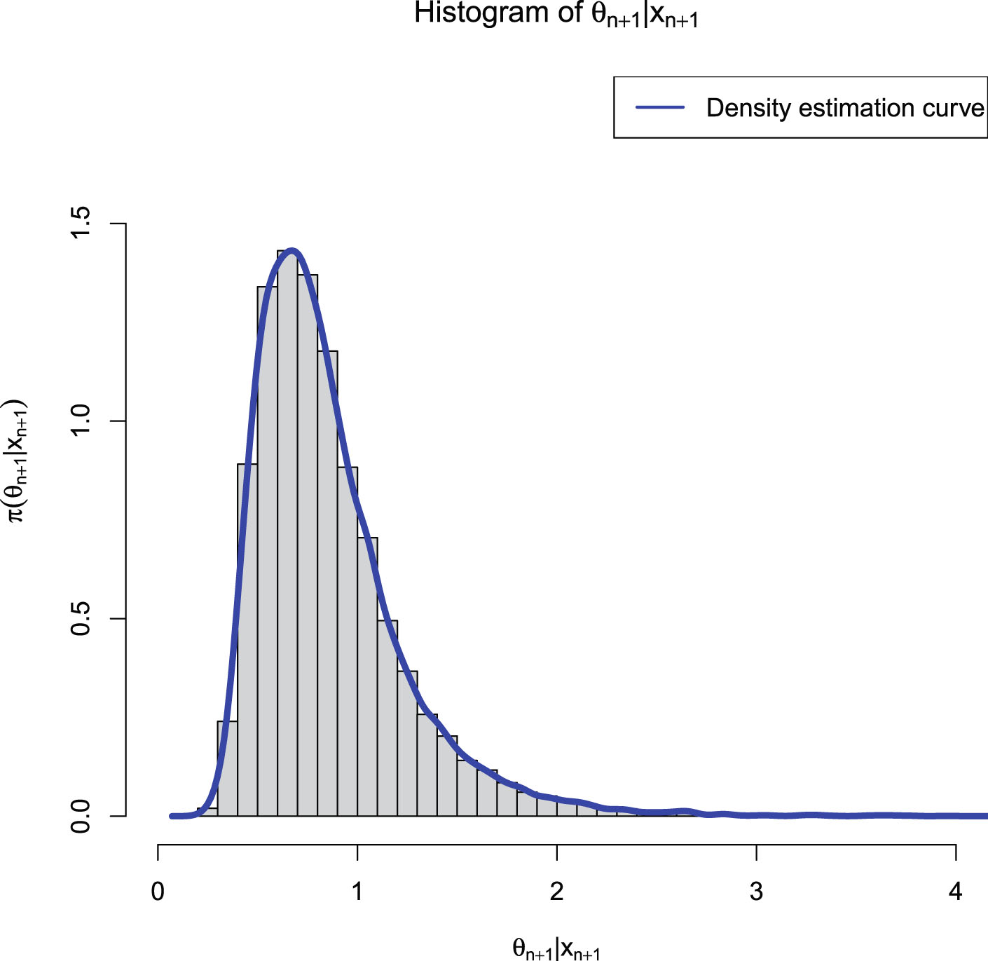
from  . Figure 2.1 shows the histogram of
  and the density estimation curve of
  . It is
  that we find
  to minimize the PESL. Numerical results show that
 and
and
 which exemplify the theoretical studies of (2.6) and (2.9).
, , and . Then we set a seed number 1 in R software and draw from . After that, we draw from . Figure 2.1 shows the histogram of and the density estimation curve of . It is that we find to minimize the PESL. Numerical results show that
FIG. 2.1 — IG-IG: The histogram of  and the density estimation curve of
  .
.
and the density estimation curve of .
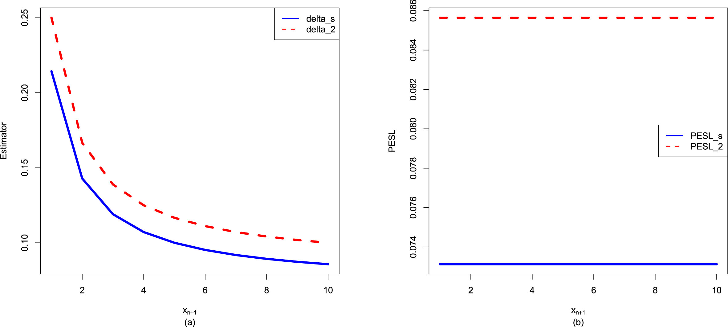
In figure 2.2, we fix  ,
,  , and
, and  , but allow
  to change from 1 to 10. From the figure, we see that the Bayes estimators and PESLs are functions of
  . The numerical values of the Bayes estimators and the PESLs in the figure are displayed in table 2.1. We see from plot (a) or the first two lines of table 2.1 that the Bayes estimators are decreasing functions of
  , and
, and  are unanimously smaller than
  , and thus (2.6) is exemplified. Plot (b) or the last two lines of table 2.1 exhibit that the PESLs do not depend on
  , and
, and  are unanimously smaller than
  , and thus (2.9) is exemplified.
, , and , but allow to change from 1 to 10. From the figure, we see that the Bayes estimators and PESLs are functions of . The numerical values of the Bayes estimators and the PESLs in the figure are displayed in table 2.1. We see from plot (a) or the first two lines of table 2.1 that the Bayes estimators are decreasing functions of , and are unanimously smaller than , and thus (2.6) is exemplified. Plot (b) or the last two lines of table 2.1 exhibit that the PESLs do not depend on , and are unanimously smaller than , and thus (2.9) is exemplified.
FIG. 2.2 — IG-IG: The Bayes estimators and the PESLs as functions of  . (a) Bayes estimators. (b) PESLs.
. (a) Bayes estimators. (b) PESLs.
TAB. 2.1 — IG-IG: The numerical values of the Bayes estimators and the PESLs in figure 2.2:  changes.
changes.
 |
1 | 2 | 3 | 4 | 5 | 6 | 7 | 8 | 9 | 10 |
 |
0.2143 | 0.1429 | 0.1190 | 0.1071 | 0.1000 | 0.0952 | 0.0918 | 0.0893 | 0.0873 | 0.0857 |
 |
0.2500 | 0.1667 | 0.1389 | 0.1250 | 0.1167 | 0.1111 | 0.1071 | 0.1042 | 0.1019 | 0.1000 |
 |
0.0731 | 0.0731 | 0.0731 | 0.0731 | 0.0731 | 0.0731 | 0.0731 | 0.0731 | 0.0731 | 0.0731 |
 |
0.0856 | 0.0856 | 0.0856 | 0.0856 | 0.0856 | 0.0856 | 0.0856 | 0.0856 | 0.0856 | 0.0856 |
Now we allow one of the three parameters  ,
,  , and
, and  to change, holding other parameters fixed. Moreover, we also assume that the datum
  is fixed, as is the case for the real data. Figure 2.3 shows the Bayes estimators and the PESLs as functions of
  ,
,  , and
, and  . We see from the left plots of the figure that the Bayes estimators depend on
  ,
,  , and
, and  , and (2.6) is exemplified. The right plots of the figure exhibit that the PESLs depend on
  and
and  , but not on
  , and (2.9) is exemplified. Furthermore, tables 2.2–2.4 display the numerical values of the Bayes estimators and the PESLs in figure 2.3. In summary, the results of figure 2.3 and tables 2.2–2.4 exemplify the theoretical studies of (2.6) and (2.9).
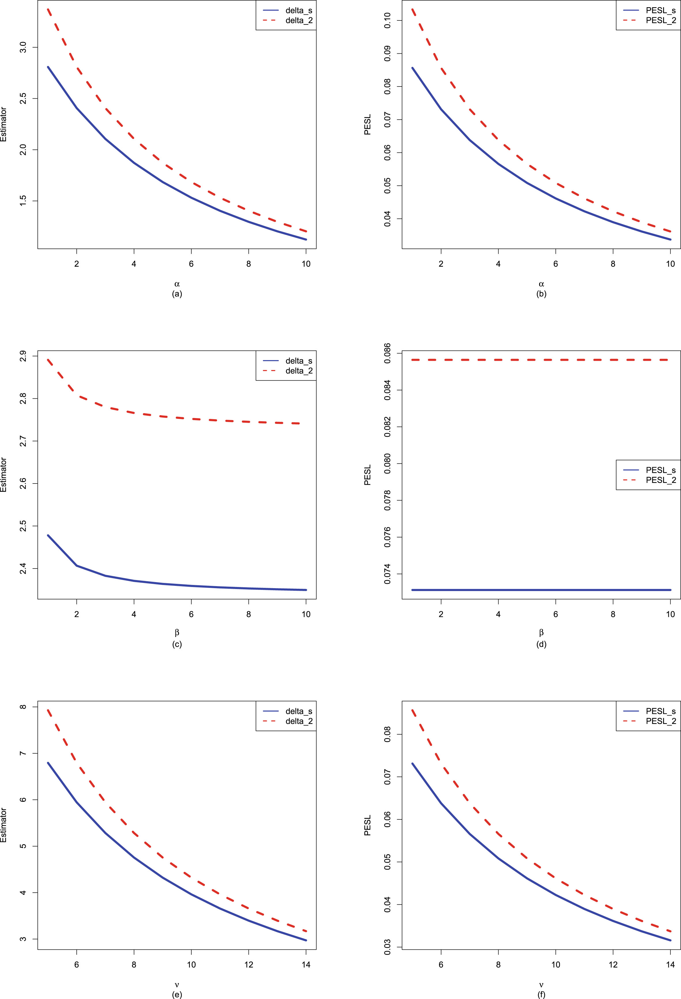
, , and to change, holding other parameters fixed. Moreover, we also assume that the datum is fixed, as is the case for the real data. Figure 2.3 shows the Bayes estimators and the PESLs as functions of , , and . We see from the left plots of the figure that the Bayes estimators depend on , , and , and (2.6) is exemplified. The right plots of the figure exhibit that the PESLs depend on and , but not on , and (2.9) is exemplified. Furthermore, tables 2.2–2.4 display the numerical values of the Bayes estimators and the PESLs in figure 2.3. In summary, the results of figure 2.3 and tables 2.2–2.4 exemplify the theoretical studies of (2.6) and (2.9).
FIG. 2.3 — IG-IG: The Bayes estimators and the PESLs as functions of  ,
,  , and
, and  . (a) Bayes estimators vs.
  . (b) PESLs vs.
  . (c) Bayes estimators vs.
  . (d) PESLs vs.
  . (e) Bayes estimators vs.
  . (f) PESLs vs.
  .
.
, , and . (a) Bayes estimators vs. . (b) PESLs vs. . (c) Bayes estimators vs. . (d) PESLs vs. . (e) Bayes estimators vs. . (f) PESLs vs. .
TAB. 2.2 — IIG-IG: The numerical values of the Bayes estimators and the PESLs in figure 2.3:  changes.
changes.
 |
1 | 2 | 3 | 4 | 5 | 6 | 7 | 8 | 9 | 10 |
 |
2.8077 | 2.4066 | 2.1058 | 1.8718 | 1.6846 | 1.5315 | 1.4038 | 1.2958 | 1.2033 | 1.1231 |
 |
3.3692 | 2.8077 | 2.4066 | 2.1058 | 1.8718 | 1.6846 | 1.5315 | 1.4038 | 1.2958 | 1.2033 |
 |
0.0856 | 0.0731 | 0.0638 | 0.0566 | 0.0508 | 0.0461 | 0.0422 | 0.0390 | 0.0361 | 0.0337 |
 |
0.1033 | 0.0856 | 0.0731 | 0.0638 | 0.0566 | 0.0508 | 0.0461 | 0.0422 | 0.0390 | 0.0361 |
TAB. 2.3 — IIG-IG: The numerical values of the Bayes estimators and the PESLs in figure 2.3:  changes.
changes.
 |
1 | 2 | 3 | 4 | 5 | 6 | 7 | 8 | 9 | 10 |
 |
2.4780 | 2.4066 | 2.3828 | 2.3709 | 2.3637 | 2.3590 | 2.3556 | 2.3530 | 2.3510 | 2.3494 |
 |
2.8910 | 2.8077 | 2.7799 | 2.7660 | 2.7577 | 2.7521 | 2.7481 | 2.7452 | 2.7429 | 2.7410 |
 |
0.0731 | 0.0731 | 0.0731 | 0.0731 | 0.0731 | 0.0731 | 0.0731 | 0.0731 | 0.0731 | 0.0731 |
 |
0.0856 | 0.0856 | 0.0856 | 0.0856 | 0.0856 | 0.0856 | 0.0856 | 0.0856 | 0.0856 | 0.0856 |
TAB. 2.4 — IIG-IG: The numerical values of the Bayes estimators and the PESLs in figure 2.3:  changes.
changes.
 |
5 | 6 | 7 | 8 | 9 | 10 | 11 | 12 | 13 | 14 |
 |
6.7943 | 5.9450 | 5.2844 | 4.7560 | 4.3236 | 3.9633 | 3.6585 | 3.3971 | 3.1707 | 2.9725 |
 |
7.9267 | 6.7943 | 5.9450 | 5.2844 | 4.7560 | 4.3236 | 3.9633 | 3.6585 | 3.3971 | 3.1707 |
 |
0.0731 | 0.0638 | 0.0566 | 0.0508 | 0.0461 | 0.0422 | 0.0390 | 0.0361 | 0.0337 | 0.0316 |
 |
0.0856 | 0.0731 | 0.0638 | 0.0566 | 0.0508 | 0.0461 | 0.0422 | 0.0390 | 0.0361 | 0.0337 |
Since the Bayes estimators  and
and  and the PESLs
  and
and  depend on
  and
and  , where
  and
and  , we can plot the surfaces of the Bayes estimators and the PESLs on the domain
  via the R function persp3d() in the R package rgl (see Adler et al. (2017)). We remark that the R function persp() in the R package graphics can not add another surface to the existing surface, but persp3d() can. Moreover, persp3d() allows one to rotate the perspective plots of the surface according to one’s wishes. Figure 2.4 plots the surfaces of the Bayes estimators and the PESLs, and the surfaces of the differences of the Bayes estimators and the PESLs. The domain for
  is
is  for all the plots. a is for
  and b is for
  in the axes of all the plots. The red surface is for
  and the blue surface is for
  in the upper two plots. From the left two plots of the figure, we see that
  for all
  on
on  . From the right two plots of the figure, we see that
  for all
  on
on  . The results of the figure exemplify the theoretical studies of (2.6) and (2.9).
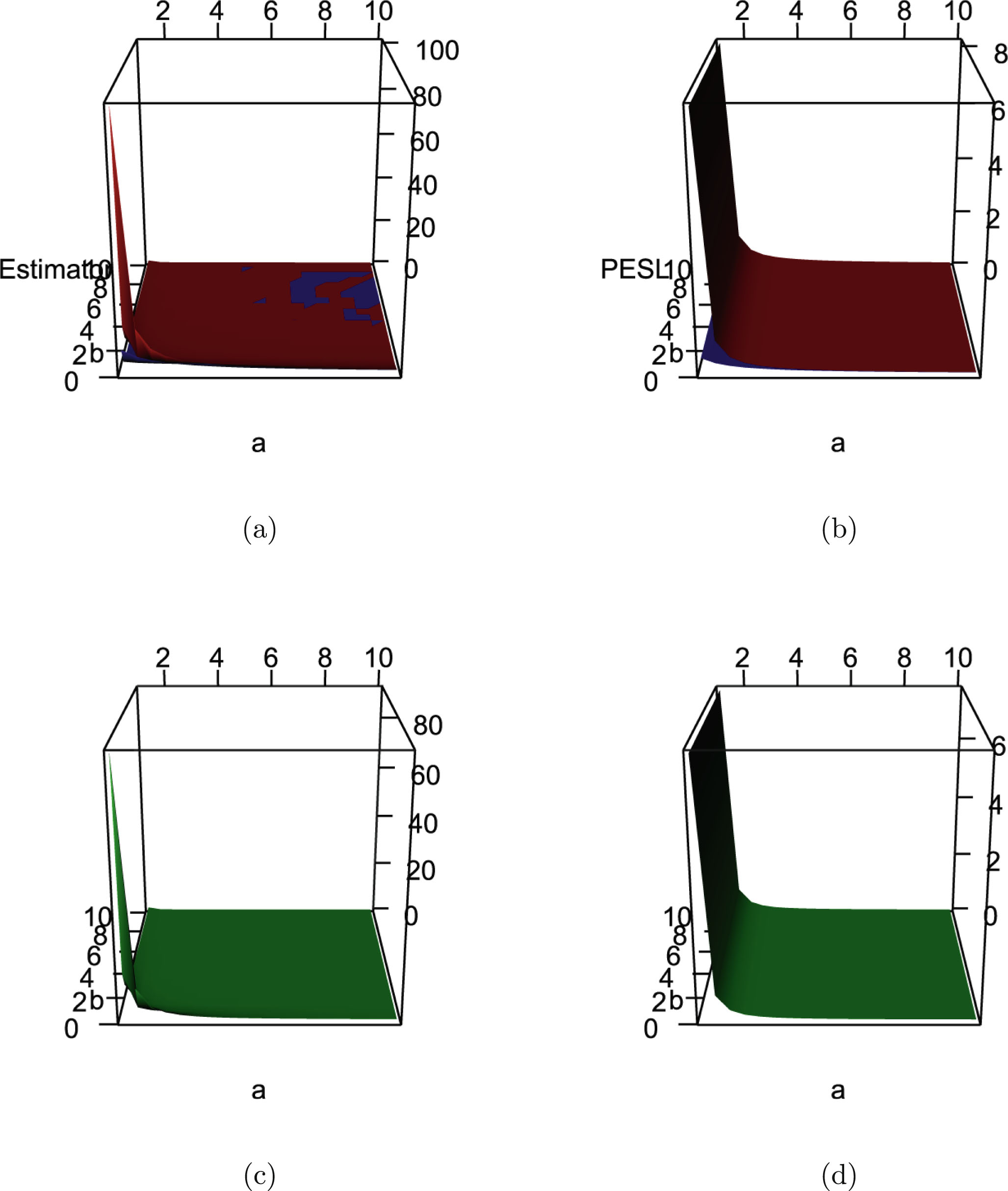
and and the PESLs and depend on and , where and , we can plot the surfaces of the Bayes estimators and the PESLs on the domain via the R function persp3d() in the R package rgl (see Adler et al. (2017)). We remark that the R function persp() in the R package graphics can not add another surface to the existing surface, but persp3d() can. Moreover, persp3d() allows one to rotate the perspective plots of the surface according to one’s wishes. Figure 2.4 plots the surfaces of the Bayes estimators and the PESLs, and the surfaces of the differences of the Bayes estimators and the PESLs. The domain for is for all the plots. a is for and b is for in the axes of all the plots. The red surface is for and the blue surface is for in the upper two plots. From the left two plots of the figure, we see that for all on . From the right two plots of the figure, we see that for all on . The results of the figure exemplify the theoretical studies of (2.6) and (2.9).
FIG. 2.4 — IG-IG: (a) The Bayes estimators as functions of  and
and  . (b) The PESLs as functions of
  and
and  . (c) The surface of
  which is positive for all
  on
on  . (d) The surface of
  which is also positive for all
  on
on  .
.
and . (b) The PESLs as functions of and . (c) The surface of which is positive for all on . (d) The surface of which is also positive for all on .
2.3.2 Consistencies of the Moment Estimators and the MLEs
In this subsection, similar to subsection 1.8.1, we will numerically exemplify that the moment estimators and the MLEs are consistent estimators of the hyperparameters  ,
,  , and
, and  of the hierarchical inverse gamma and inverse gamma model (2.1). The motivation of this subsection is that in Theorems 2.2 and 2.3, we have theoretically shown that the moment estimators and the MLEs are consistent estimators of the hyperparameters. Note that only
  are used in this subsection. The simulation design of this subsection is detailed in appendix A.4.
, , and of the hierarchical inverse gamma and inverse gamma model (2.1). The motivation of this subsection is that in Theorems 2.2 and 2.3, we have theoretically shown that the moment estimators and the MLEs are consistent estimators of the hyperparameters. Note that only are used in this subsection. The simulation design of this subsection is detailed in appendix A.4.
The frequencies of the moment estimators ( ,
,  , and
, and  ) and the MLEs (
 ,
,  , and
, and  ) of the hyperparameters (
 ,
,  , and
, and  ) as
) as  varies for
  and
and  , 0.5, and 0.1 are reported in table 2.5. From this table, we observe the following facts.
, , and ) and the MLEs (, , and ) of the hyperparameters (, , and ) as varies for and , 0.5, and 0.1 are reported in table 2.5. From this table, we observe the following facts.
1. Given  , 0.5, or 0.1, the frequencies of the estimators (
 ,
,  ,
,  , or
, or  ,
,  ) tend to 0 as
  increases to infinity, which means that the moment estimators and the MLEs are consistent estimators of the hyperparameters. For
  , the frequencies of the estimators are still very large. However, we observe the tendencies of declining to 0 as
  increases to infinity.
, 0.5, or 0.1, the frequencies of the estimators (, , , or , ) tend to 0 as increases to infinity, which means that the moment estimators and the MLEs are consistent estimators of the hyperparameters. For , the frequencies of the estimators are still very large. However, we observe the tendencies of declining to 0 as increases to infinity.
2. Comparing the frequencies corresponding to  , 0.5, and 0.1, we observe that as
  gets smaller, the frequencies tend to be larger, since the constraints
 are easier to meet.
, 0.5, and 0.1, we observe that as gets smaller, the frequencies tend to be larger, since the constraints
3. Comparing the moment estimators and the MLEs of the hyperparameters  ,
,  , and
, and  , we see that the frequencies of the MLEs are smaller than those of the moment estimators, which means that the MLEs are better than the moment estimators when estimating the hyperparameters in terms of consistency.
, , and , we see that the frequencies of the MLEs are smaller than those of the moment estimators, which means that the MLEs are better than the moment estimators when estimating the hyperparameters in terms of consistency.
TAB. 2.5 — IIG-IG: The frequencies of the moment estimators and the MLEs of the hyperparameters as  varies for
  and
and  , 0.5, and 0.1.
varies for and , 0.5, and 0.1.
| Moment estimators | MLEs | ||||||
| n |  |
 |
 |
 |
 |
 |
|
 |
1e4 | 0.01 | 0.25 | 0.33 | 0.01 | 0.03 | 0.04 |
| 2e4 | 0.00 | 0.09 | 0.12 | 0.00 | 0.00 | 0.01 | |
| 4e4 | 0.00 | 0.01 | 0.07 | 0.00 | 0.00 | 0.00 | |
| 8e4 | 0.00 | 0.00 | 0.00 | 0.00 | 0.00 | 0.00 | |
 |
1e4 | 0.07 | 0.62 | 0.63 | 0.05 | 0.07 | 0.12 |
| 2e4 | 0.05 | 0.55 | 0.60 | 0.02 | 0.05 | 0.07 | |
| 4e4 | 0.03 | 0.45 | 0.48 | 0.01 | 0.06 | 0.09 | |
| 8e4 | 0.01 | 0.20 | 0.27 | 0.00 | 0.01 | 0.02 | |
 |
1e4 | 0.82 | 0.94 | 0.88 | 0.14 | 0.56 | 0.75 |
| 2e4 | 0.83 | 0.92 | 0.93 | 0.09 | 0.40 | 0.65 | |
| 4e4 | 0.71 | 0.92 | 0.90 | 0.10 | 0.32 | 0.53 | |
| 8e4 | 0.62 | 0.87 | 0.88 | 0.07 | 0.19 | 0.34 | |
2.3.3 Goodness-of-Fit of the Model: KS Test
In this subsection, similar to subsection 1.8.2, we will calculate the goodness-of-fit of the hierarchical inverse gamma and inverse gamma model (2.1) to the simulated data. The motivation of this subsection is that we want to check whether the marginal distribution of the hierarchical inverse gamma and inverse gamma model (2.1) fits the simulated data well. Note that only  are used in this subsection.
are used in this subsection.
In our problem, the null hypothesis specifies that
 where
where  is the marginal distribution of the hierarchical inverse gamma and inverse gamma model (2.1). The marginal density of the
  distribution is given by (2.3), which is obviously one-dimensional continuous. Hence, the KS test can be utilized as a measure of the goodness-of-fit.
is the marginal distribution of the hierarchical inverse gamma and inverse gamma model (2.1). The marginal density of the distribution is given by (2.3), which is obviously one-dimensional continuous. Hence, the KS test can be utilized as a measure of the goodness-of-fit.
The results of the KS test goodness-of-fit of the model (2.1) to the simulated data are reported in table 2.6. Note that the data are simulated according to the hierarchical inverse gamma and inverse gamma model (2.1) with  ,
,  , and
, and  . In the table, the hyperparameters
  ,
,  , and
, and  are estimated by three methods. The first method is the oracle method, in that we know the hyperparameters
  ,
,  , and
, and  . The second method is the moment method, in that the hyperparameters
  ,
,  , and
, and  are estimated by their moment estimators (see Theorem 2.2). The third method is the MLE method, in that the hyperparameters
  ,
,  , and
, and  are estimated by their MLEs (see Theorem 2.3). In the table, the sample size is
  , and the number of simulations is
  .
.
, , and . In the table, the hyperparameters , , and are estimated by three methods. The first method is the oracle method, in that we know the hyperparameters , , and . The second method is the moment method, in that the hyperparameters , , and are estimated by their moment estimators (see Theorem 2.2). The third method is the MLE method, in that the hyperparameters , , and are estimated by their MLEs (see Theorem 2.3). In the table, the sample size is , and the number of simulations is .
1. From table 2.6, we observe the following facts.
The  values for the three methods are respectively given by 0.2983, 0.0338, and 0.0255, which means that the MLE method is the best method, the moment method is the second-best method, and the oracle method is the worst method. A possible explanation for this phenomenon is that in (1.23), the empirical cdf
  is based on data, and the population cdfs
  for the MLE method and the moment method are also based on data, while the population cdf
  for the oracle method is not based on data.
values for the three methods are respectively given by 0.2983, 0.0338, and 0.0255, which means that the MLE method is the best method, the moment method is the second-best method, and the oracle method is the worst method. A possible explanation for this phenomenon is that in (1.23), the empirical cdf is based on data, and the population cdfs for the MLE method and the moment method are also based on data, while the population cdf for the oracle method is not based on data.
2. The  values for the three methods are respectively given by 0.0677, 0.4077, and 0.6503, which also means that the MLE method ranks first, the moment method ranks second, and the oracle method ranks third. The possible explanation for this phenomenon is described in the previous paragraph.
values for the three methods are respectively given by 0.0677, 0.4077, and 0.6503, which also means that the MLE method ranks first, the moment method ranks second, and the oracle method ranks third. The possible explanation for this phenomenon is described in the previous paragraph.
3. The  values for the three methods are respectively given by 0.02, 0.40, and 0.58. The
  value for the MLE method accounts for over half of the
  simulations. The order of preference for the three methods is the MLE method, the moment method, and the oracle method.
values for the three methods are respectively given by 0.02, 0.40, and 0.58. The value for the MLE method accounts for over half of the simulations. The order of preference for the three methods is the MLE method, the moment method, and the oracle method.
4. The  values for the three methods are respectively given by 0.02, 0.40, and 0.58. A small
  value corresponds to a large p-value. Hence, the smallest
  value corresponds to the largest p-value. Therefore, the
  value and the
  value for the three methods are the same. The order of preference for the three methods is the MLE method, the moment method, and the oracle method.
values for the three methods are respectively given by 0.02, 0.40, and 0.58. A small value corresponds to a large p-value. Hence, the smallest value corresponds to the largest p-value. Therefore, the value and the value for the three methods are the same. The order of preference for the three methods is the MLE method, the moment method, and the oracle method.
5. The  values for the three methods are respectively given by 0.14, 0.81, and 0.91. Once again, the order of preference for the three methods is the MLE method, the moment method, and the oracle method. The
  values for the moment method and the MLE method are over
  , which means that the two methods have good performances in terms of goodness-of-fit.
values for the three methods are respectively given by 0.14, 0.81, and 0.91. Once again, the order of preference for the three methods is the MLE method, the moment method, and the oracle method. The values for the moment method and the MLE method are over , which means that the two methods have good performances in terms of goodness-of-fit.
6. In summary, for the five indices ( ,
,  ,
,  ,
,  ,
,  ), the order of preference for the three methods is the MLE method, the moment method, and the oracle method. Comparing the moment method and the MLE method, we find that the MLE method has a better performance than the moment method in terms of all five indices.
, , , , ), the order of preference for the three methods is the MLE method, the moment method, and the oracle method. Comparing the moment method and the MLE method, we find that the MLE method has a better performance than the moment method in terms of all five indices.
TAB. 2.6 — IIG-IG: The results of the KS test goodness-of-fit of the model (2.1) to the simulated data.
| Oracle method | Moment method | MLE method | |
 |
0.2983 | 0.0338 | 0.0255 |
 |
0.0677 | 0.4077 | 0.6503 |
 |
0.02 | 0.40 | 0.58 |
 |
0.02 | 0.40 | 0.58 |
 |
0.14 | 0.81 | 0.91 |
The boxplots of the  values and the p-values for the three methods are displayed in figure 2.5. From the figure, we observe the following facts.
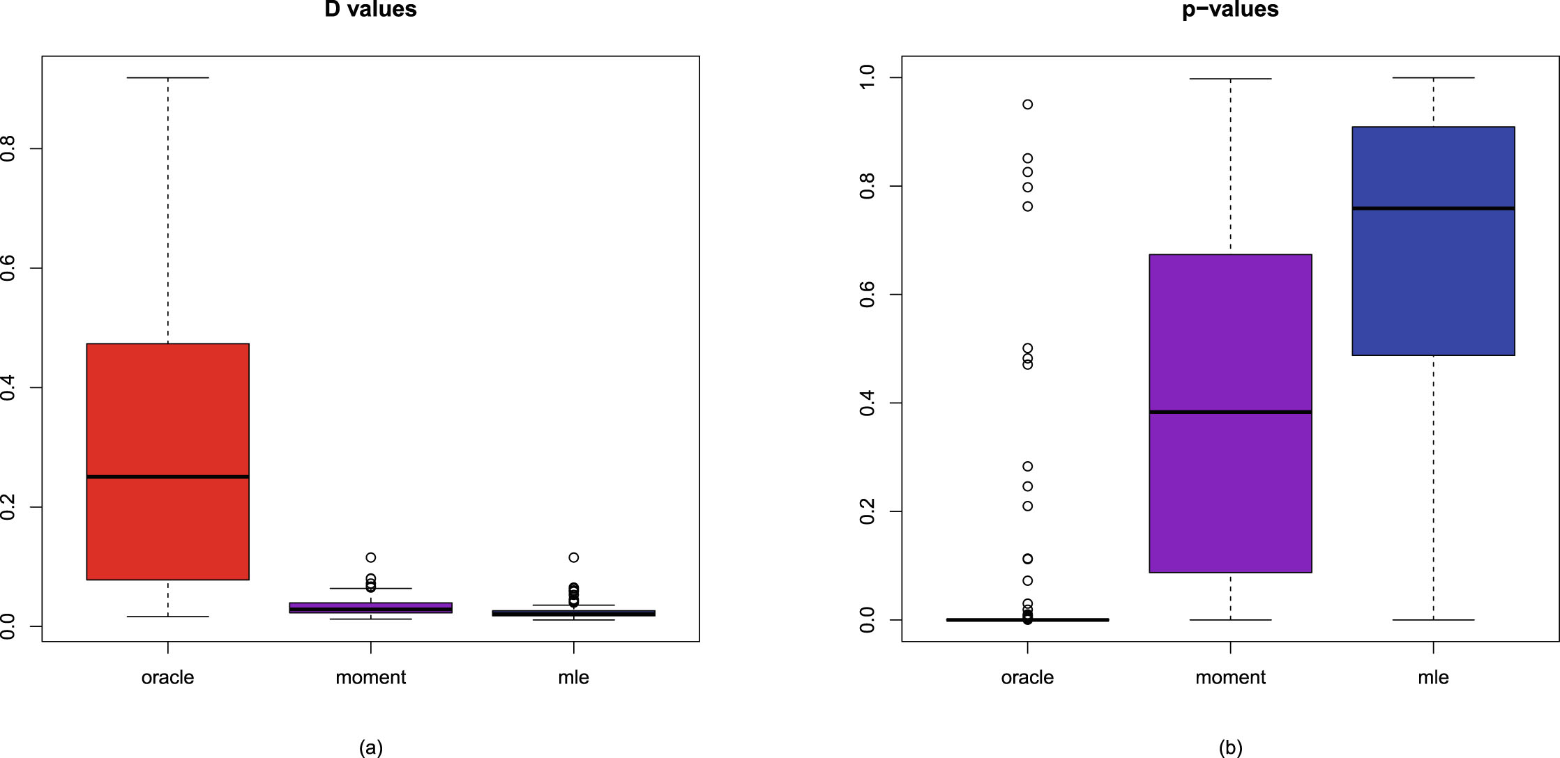
values and the p-values for the three methods are displayed in figure 2.5. From the figure, we observe the following facts.
1. The  values of the oracle method are significantly larger than those of the other two methods. Since for the
  value, the smaller the better, the order of preference for the three methods is the MLE method, the moment method, and the oracle method.
values of the oracle method are significantly larger than those of the other two methods. Since for the value, the smaller the better, the order of preference for the three methods is the MLE method, the moment method, and the oracle method.
2. The p-values of the oracle method are significantly smaller than those of the other two methods. Since for the p-value, the larger the better, the order of preference for the three methods is the MLE method, the moment method, and the oracle method.
3. Small  values correspond to large p-values, and large
  values correspond to small p-values.
values correspond to large p-values, and large values correspond to small p-values.
4. The MLE method has a better performance than the moment method in terms of the  values and the p-values.
values and the p-values.
FIG. 2.5 — IG-IG: The boxplots of the  values and the p-values for the three methods. (a)
  values. (b) p-values.
values and the p-values for the three methods. (a) values. (b) p-values.
2.3.4 Numerical Comparisons of the Bayes Estimators and the PESLs of Three Methods
In this subsection, we will numerically compare the Bayes estimators and the PESLs of the three methods (the oracle method, the moment method, and the MLE method). The motivation of this subsection is that the theoretical comparisons of the Bayes estimators and the PESLs of the three methods can be found in subsection 2.2.3. Note that the full data  are used in this subsection.
are used in this subsection.
Note that the data are simulated according to the hierarchical inverse gamma and inverse gamma model (2.1) with  ,
,  , and
, and  . Moreover, the oracle method knows the hyperparameters
  ,
,  , and
, and  in simulations.
, , and . Moreover, the oracle method knows the hyperparameters , , and in simulations.
Comparisons of the Bayes estimators and the PESLs of the three methods for sample size  and number of simulations
  are displayed in figure 2.6. From the figure, we observe the following facts.
and number of simulations are displayed in figure 2.6. From the figure, we observe the following facts.
1. Plot (a): For the Bayes estimators of  under Stein’s loss function
 , the MLE method is slightly closer to the oracle method than the moment method.
under Stein’s loss function , the MLE method is slightly closer to the oracle method than the moment method.
2. Plot (b): For the Bayes estimators of  under the squared error loss function
 , the MLE method is also slightly closer to the oracle method than the moment method.
under the squared error loss function , the MLE method is also slightly closer to the oracle method than the moment method.
3. Plot (c): For the PESLs 
 , the MLE method is much closer to the oracle method than the moment method.
, the MLE method is much closer to the oracle method than the moment method.
4. Plot (d): For the PESLs 
 , the MLE method is also much closer to the oracle method than the moment method.
, the MLE method is also much closer to the oracle method than the moment method.
5. All four plots indicate that the MLE method is better than the moment method, as the Bayes estimators and the PESLs of the MLE method are closer to those of the oracle method than those of the moment method.
The boxplots of the absolute errors from the oracle method by the moment method, and the MLE method for sample size  and number of simulations
  are displayed in figure 2.7. All four plots indicate that the MLE method is better than the moment method, as the absolute errors from the oracle method of the Bayes estimators and the PESLs by the MLE method are much smaller than those of the moment method.
and number of simulations are displayed in figure 2.7. All four plots indicate that the MLE method is better than the moment method, as the absolute errors from the oracle method of the Bayes estimators and the PESLs by the MLE method are much smaller than those of the moment method.
The averages and proportions of the absolute errors from the oracle method by the moment method, and the MLE method for the Bayes estimators and the PESLs are summarized in table 2.7. See Subsection 1.8.3 for details. From the table, we observe that the averages of the absolute errors from the oracle method by the MLE method are much smaller than those by the moment method. Moreover, the proportions of the absolute errors from the oracle method by the MLE method are much larger than those by the moment method. In summary, the table illustrates that the MLE method is better than the moment method in terms of the averages and proportions of the absolute errors from the oracle method.
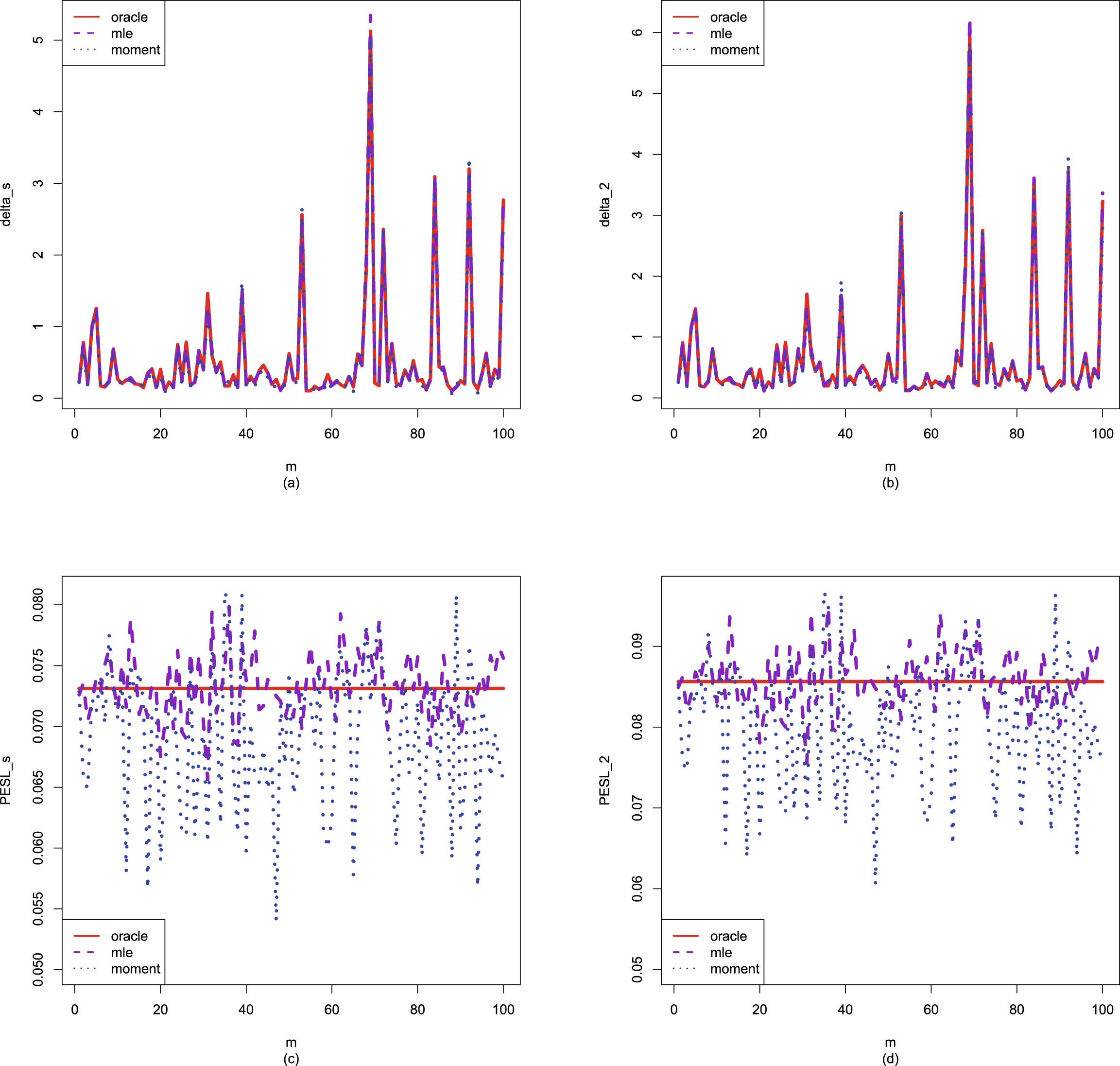
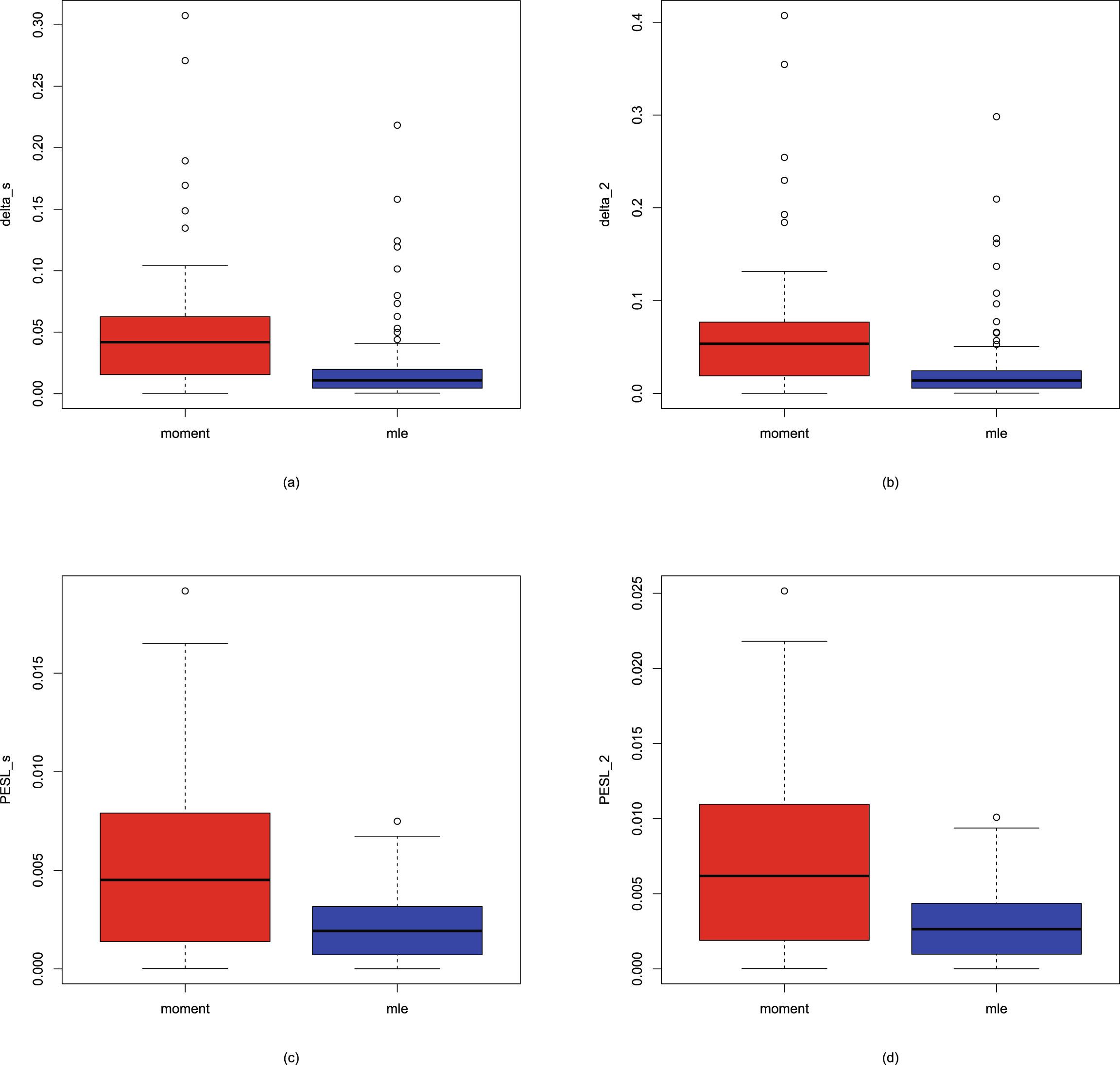
FIG. 2.6 — IG-IG: Comparisons of the Bayes estimators and the PESLs of the three methods for sample size  and number of simulations
  . (a)
. (a) 
 . (b)
. (b) 
 . (c)
. (c) 
 . (d)
. (d) 
 .
.
and number of simulations . (a) . (b) . (c) . (d) .
FIG. 2.7 — IG-IG: The boxplots of the absolute errors from the oracle method by the moment method, and the MLE method for sample size  and number of simulations
  . (a) Absolute errors for
  . (b) Absolute errors for
  . (c) Absolute errors for
  . (d) Absolute errors for
  .
.
and number of simulations . (a) Absolute errors for . (b) Absolute errors for . (c) Absolute errors for . (d) Absolute errors for .
TAB. 2.7 — IIG-IG: The averages and proportions of the absolute errors from the oracle method by the moment method and the MLE method for the Bayes estimators and the PESLs.
| Averages | Proportions | |||
| Moment | MLE | Moment | MLE | |
 |
0.0491 | 0.0210 | 0.20 | 0.80 |
 |
0.0626 | 0.0275 | 0.21 | 0.79 |
 |
0.0056 | 0.0022 | 0.29 | 0.71 |
 |
0.0075 | 0.0030 | 0.29 | 0.71 |
2.3.5 Marginal Densities for Various Hyperparameters
In this subsection, we will plot the marginal densities of the hierarchical inverse gamma and inverse gamma model (2.1) for various hyperparameters  ,
,  , and
, and  . The motivation of this subsection is that we want to know what kind of data can be modeled by the hierarchical inverse gamma and inverse gamma model (2.1). Note that the marginal density of
  is given by (2.3) specified by three hyperparameters
  ,
,  , and
, and  . We will explore how the marginal densities change around the marginal density with hyperparameters specified by
  ,
,  , and
, and  . Other numerical values of the hyperparameters can also be specified.
, , and . The motivation of this subsection is that we want to know what kind of data can be modeled by the hierarchical inverse gamma and inverse gamma model (2.1). Note that the marginal density of is given by (2.3) specified by three hyperparameters , , and . We will explore how the marginal densities change around the marginal density with hyperparameters specified by , , and . Other numerical values of the hyperparameters can also be specified.
Figure 2.8 plots the marginal densities for varied  , holding
  and
and  fixed. From the figure, we see that as
  increases, the peak value of the curve decreases. In other words, the variance of the marginal density increases as
 (2.16)
is an increasing function of
(2.16)
is an increasing function of  . Moreover, all the marginal densities are right-skewed.
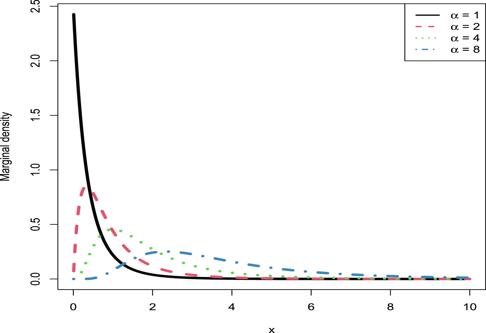
, holding and fixed. From the figure, we see that as increases, the peak value of the curve decreases. In other words, the variance of the marginal density increases as
(2.16)
. Moreover, all the marginal densities are right-skewed.
FIG. 2.8 — IG-IG: The marginal densities for varied  , holding
  and
and  fixed.
, holding and fixed.
Figure 2.9 plots the marginal densities for varied  , holding
  and
and  fixed. From the figure, we also see that as
  increases, the peak value of the curve decreases. In other words, the variance of the marginal density increases, as (2.16) is an increasing function of
  . Moreover, all the marginal densities are also right-skewed.
, holding and fixed. From the figure, we also see that as increases, the peak value of the curve decreases. In other words, the variance of the marginal density increases, as (2.16) is an increasing function of . Moreover, all the marginal densities are also right-skewed.
Figure 2.10 plots the marginal densities for varied  , holding
  and
and  fixed. From the figure, we see that as
  increases, the peak value of the curve increases. In other words, the variance of the marginal density decreases, as (2.16) is a decreasing function of
  . Moreover, all the marginal densities are also right-skewed.
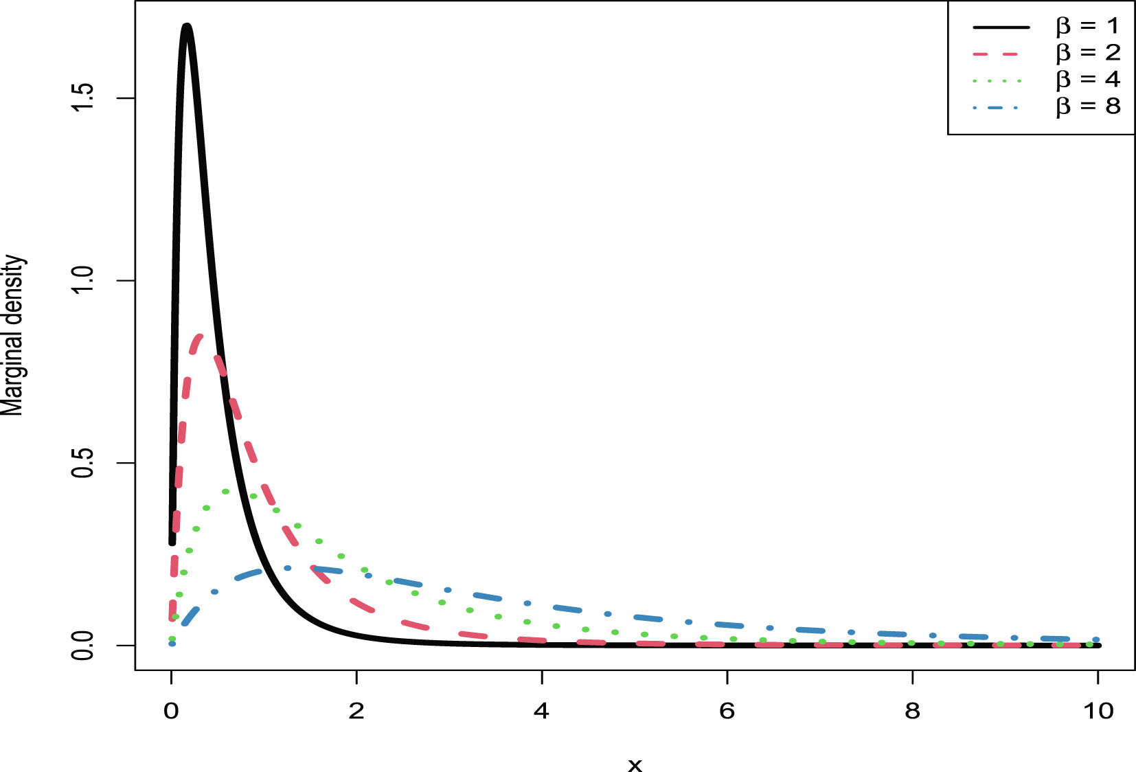
, holding and fixed. From the figure, we see that as increases, the peak value of the curve increases. In other words, the variance of the marginal density decreases, as (2.16) is a decreasing function of . Moreover, all the marginal densities are also right-skewed.
FIG. 2.9 — IG-IG: The marginal densities for varied  , holding
  and
and  fixed.
, holding and fixed.
2.4 Conclusions and Discussions
For the hierarchical inverse gamma and inverse gamma model (2.1), we calculate the posterior density  and the marginal density
  in Theorem 2.1. Since
  is a rate parameter in (2.1), the Bayes estimator of
  under the squared error loss function is not appropriate. In contrast, we should choose Stein’s loss function because it penalizes gross overestimation and gross underestimation equally. After that, we calculate the Bayes estimators of
  ,
,  and
and  , and the PESLs of
  ,
,  and
and  .
.
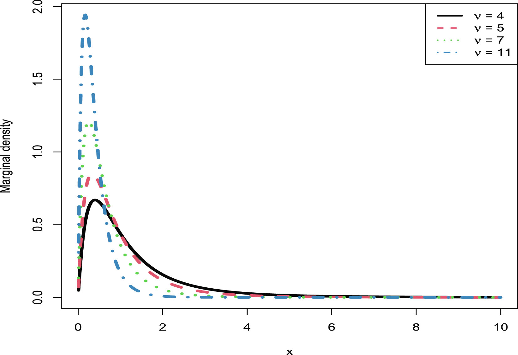
and the marginal density in Theorem 2.1. Since is a rate parameter in (2.1), the Bayes estimator of under the squared error loss function is not appropriate. In contrast, we should choose Stein’s loss function because it penalizes gross overestimation and gross underestimation equally. After that, we calculate the Bayes estimators of , and , and the PESLs of , and .
FIG. 2.10 — IG-IG: The marginal densities for varied  , holding
  and
and  fixed.
, holding and fixed.
In order to calculate the empirical Bayes estimator of the rate parameter  , we must calculate the estimators of the hyperparameters of model (2.1). The estimators of the hyperparameters of model (2.1) by the moment method and their consistencies are summarized in Theorem 2.2. Moreover, the estimators of the hyperparameters of model (2.1) by the MLE method and their consistencies are summarized in Theorem 2.3. Finally, the empirical Bayes estimators of the rate parameter
  of the model (2.1) under Stein’s loss function by the moment method and the MLE method are summarized in Theorem 2.4.
, we must calculate the estimators of the hyperparameters of model (2.1). The estimators of the hyperparameters of model (2.1) by the moment method and their consistencies are summarized in Theorem 2.2. Moreover, the estimators of the hyperparameters of model (2.1) by the MLE method and their consistencies are summarized in Theorem 2.3. Finally, the empirical Bayes estimators of the rate parameter of the model (2.1) under Stein’s loss function by the moment method and the MLE method are summarized in Theorem 2.4.
Note that in Theorem 2.3, we only stated that the estimators of the hyperparameters of model (2.1) by the MLE method  ,
,  , and
, and  are the solutions to the equations (2.13)–(2.15). We can exploit Newton’s method to solve the equations (2.13)–(2.15) and to numerically obtain the MLEs of
  ,
,  , and
, and  . However, we can not prove the existence and uniqueness of the solutions to our system. The interested readers who have such kind of knowledge and skills are encouraged to solve this issue.
, , and are the solutions to the equations (2.13)–(2.15). We can exploit Newton’s method to solve the equations (2.13)–(2.15) and to numerically obtain the MLEs of , , and . However, we can not prove the existence and uniqueness of the solutions to our system. The interested readers who have such kind of knowledge and skills are encouraged to solve this issue.
Numerical simulations illustrate that the moment estimators ( ,
,  , and
, and  ) and the MLEs (
 ,
,  , and
, and  ) are consistent estimators of the hyperparameters (
 ,
,  , and
, and  ), as reported in table 2.5. Moreover, table 2.6 indicates that the hierarchical inverse gamma and inverse gamma model (2.1) fits the simulated data well in terms of the KS test goodness-of-fit by the moment method and the MLE method.
, , and ) and the MLEs (, , and ) are consistent estimators of the hyperparameters (, , and ), as reported in table 2.5. Moreover, table 2.6 indicates that the hierarchical inverse gamma and inverse gamma model (2.1) fits the simulated data well in terms of the KS test goodness-of-fit by the moment method and the MLE method.
The plots of the marginal densities show that all the curves are right-skewed. Therefore, the hierarchical inverse gamma and inverse gamma model (2.1) could potentially be used to fit right-skewed data, not left-skewed data.
It is common to assume that the variance parameter (or positive parameter) follows an inverse gamma distribution. Therefore, the hierarchical inverse gamma and inverse gamma model (2.1), as a more variable inverse gamma distribution, could be used to model the variance parameter (or positive parameter).
Chapter 3 The Empirical Bayes Estimators of the Rate Parameter of the Gamma Distribution with a Conjugate Gamma Prior under Stein’s Loss Function
For the hierarchical gamma and gamma model, we calculate the Bayes estimator of the rate parameter of the gamma distribution under Stein’s loss function, which penalizes gross overestimation and gross underestimation equally, and the corresponding PESL. We also obtain the Bayes estimator of the rate parameter under the squared error loss function and the corresponding PESL. Moreover, we obtain the empirical Bayes estimators of the rate parameter of the gamma distribution with a conjugate gamma prior by the moment and MLE methods under Stein’s loss function. In numerical simulations, we have illustrated five aspects: The two inequalities of the Bayes estimators and the PESLs for the oracle method; the moment estimators and the MLEs are consistent estimators of the hyperparameters; the goodness-of-fit of the model to the simulated data; the comparisons of the Bayes estimators and the PESLs of the oracle, moment, and MLE methods; and the marginal densities of the model for various hyperparameters. The numerical results indicate that the MLEs are better than the moment estimators when estimating the hyperparameters. Finally, the hierarchical gamma and gamma model could potentially be used to fit right-skewed data, not left-skewed data.
Acknowledgement. This chapter is derived in part from an article Shi et al. (2025) published in Communications in Statistics-Simulation and Computation 22 June 2024 <copyright Taylor & Francis>, available online: http://www.tandfonline.com/10.1080/03610918.2024.2369811.
3.1 Introduction
The hierarchical gamma and gamma model (3.1) has been considered in table 3.3.1 (p. 121) and table 4.2.1 (p. 176) of Robert (2007). However, he only calculated the Bayes estimator of  under the squared error loss function. Since the rate parameter
  is a positive parameter, the Bayes estimator of
  under the squared error loss function is not appropriate. In contrast, we should choose Stein’s loss function (James and Stein (1961); see also Brown (1990)) because it penalizes gross overestimation and gross underestimation equally. To determine the unknown hyperparameters, we adopt the empirical Bayes method. In this chapter, we calculate the Bayes estimator of
  under Stein’s loss function and the corresponding PESL. We also obtain the Bayes estimator of
  under the squared error loss function and the corresponding PESL. Moreover, we obtain the empirical Bayes estimators of the rate parameter
  of the gamma distribution with a conjugate gamma prior by the moment method and the MLE method under Stein’s loss function.
under the squared error loss function. Since the rate parameter is a positive parameter, the Bayes estimator of under the squared error loss function is not appropriate. In contrast, we should choose Stein’s loss function (James and Stein (1961); see also Brown (1990)) because it penalizes gross overestimation and gross underestimation equally. To determine the unknown hyperparameters, we adopt the empirical Bayes method. In this chapter, we calculate the Bayes estimator of under Stein’s loss function and the corresponding PESL. We also obtain the Bayes estimator of under the squared error loss function and the corresponding PESL. Moreover, we obtain the empirical Bayes estimators of the rate parameter of the gamma distribution with a conjugate gamma prior by the moment method and the MLE method under Stein’s loss function.
The rest of the chapter is organized as follows. In section 3.2, we calculate the Bayes estimators and the PESLs, and they satisfy two inequalities (3.6) and (3.9). Moreover, we summarize the empirical Bayes estimators of the parameter of the model (3.1) under Stein’s loss function by the moment method and the MLE method in Theorem 3.4. Furthermore, we have theoretically compared the Bayes estimators and the PESLs of the three methods (the oracle method, the moment method, and the MLE method). In section 3.3, we will carry out some numerical simulations, where we will illustrate five aspects. First, we will numerically exemplify the two inequalities of the Bayes estimators and the PESLs for the oracle method. Second, we will illustrate that the moment estimators and the MLEs are consistent estimators of the hyperparameters. Third, we will calculate the goodness-of-fit of the model (3.1) to the simulated data. Fourth, we will numerically compare the Bayes estimators and the PESLs of the three methods. Finally, we will plot the marginal densities of the hierarchical gamma and gamma model (3.1) for various hyperparameters. Some conclusions and discussions are provided in section 3.4.
3.2 Theoretical Results
Suppose that we observe  from the hierarchical gamma and gamma model:
 (3.1)
where
(3.1)
where  ,
,  , and
, and  are hyperparameters to be estimated,
  is the unknown parameter of interest,
  is the gamma distribution with shape parameter
  and rate parameter
  , and
, and  is the gamma distribution with shape parameter
  and rate parameter
  . As described in Deely and Lindley (1981), the statistician observes data
  and wishes to make an inference about
  . Therefore,
  provides direct information about the parameter
  , while supplementary information
  is also available. The connection between the prime data
  and the supplementary information
  is provided by the common distributions
  and
and  . The pdfs of
  and
and  can be found in section 1.2.
from the hierarchical gamma and gamma model:
(3.1)
, , and are hyperparameters to be estimated, is the unknown parameter of interest, is the gamma distribution with shape parameter and rate parameter , and is the gamma distribution with shape parameter and rate parameter . As described in Deely and Lindley (1981), the statistician observes data and wishes to make an inference about . Therefore, provides direct information about the parameter , while supplementary information is also available. The connection between the prime data and the supplementary information is provided by the common distributions and . The pdfs of and can be found in section 1.2.
Now we give the justifications of why  is the only parameter of interest. The pdf of
  is
is
 for
for  and
and  . We can only handle the case of an unknown rate parameter
  , letting the shape parameter
  be a hyperparameter to be determined. If the shape parameter
  is also an unknown parameter of interest, then we have to deal with the
  part in the posterior distribution, which is very complicated and has no analytical solutions. It seems that the Bayesian community avoids dealing with such a situation by letting
  be a known constant or assuming
  be a hyperparameter to be determined.
is the only parameter of interest. The pdf of is
and . We can only handle the case of an unknown rate parameter , letting the shape parameter be a hyperparameter to be determined. If the shape parameter is also an unknown parameter of interest, then we have to deal with the part in the posterior distribution, which is very complicated and has no analytical solutions. It seems that the Bayesian community avoids dealing with such a situation by letting be a known constant or assuming be a hyperparameter to be determined.
3.2.1 The Bayes Estimators and the PESLs
For the hierarchical gamma and gamma model (3.1), the posterior density of  and the marginal density of
  are given by the following theorem, whose proof can be found in appendix A.5.
and the marginal density of are given by the following theorem, whose proof can be found in appendix A.5.
Theorem 3.1. For the hierarchical gamma and gamma model (3.1), the posterior density of  is
is
 where
where
 (3.2)
(3.2)
is
(3.2)
Moreover, the marginal density of  is
is
 (3.3)
for
(3.3)
for  and
and  .
.
is
(3.3)
and .
From Theorem 3.1, we have

Since  is a rate parameter of the gamma distribution, the Bayes estimator of
  under the squared error loss function is not appropriate. In contrast, we should choose Stein’s loss function because it penalizes gross overestimation and gross underestimation equally. From (1.12), the Bayes estimator of
  under Stein’s loss function is given by
 (3.4)
for
(3.4)
for  , where
  and
and  are given by (3.2). Moreover, from (1.13), the Bayes estimator of
  under the usual squared error loss function is given by
 (3.5)
(3.5)
is a rate parameter of the gamma distribution, the Bayes estimator of under the squared error loss function is not appropriate. In contrast, we should choose Stein’s loss function because it penalizes gross overestimation and gross underestimation equally. From (1.12), the Bayes estimator of under Stein’s loss function is given by
(3.4)
, where and are given by (3.2). Moreover, from (1.13), the Bayes estimator of under the usual squared error loss function is given by
(3.5)
It is easy to see that
 (3.6)
which exemplifies the theoretical study of (1.16). Furthermore, from (1.14) and (1.15), the PESLs at
(3.6)
which exemplifies the theoretical study of (1.16). Furthermore, from (1.14) and (1.15), the PESLs at  and
and  are respectively given by
 (3.7)
and
(3.7)
and
 (3.8)
where
(3.8)
where
 is the digamma function. It is worth noting that the two PESLs
  and
and  ) depend on
  , which is given by

(3.6)
and are respectively given by
(3.7)
(3.8)
and ) depend on , which is given by
The calculations of  and the two PESLs can be found in appendix A.6. It is easy to show that
 (3.9)
which exemplifies the theoretical study of (1.17). The numerical simulations will exemplify (3.6) and (3.9).
(3.9)
which exemplifies the theoretical study of (1.17). The numerical simulations will exemplify (3.6) and (3.9).
and the two PESLs can be found in appendix A.6. It is easy to show that
(3.9)
It is worth noting that the Bayes estimators and the PESLs in this subsection assume that the hyperparameters  ,
,  , and
, and  are known. In other words, the Bayes estimators and the PESLs in this subsection are calculated by the oracle method, which will be further discussed in subsection 3.2.3.
, , and are known. In other words, the Bayes estimators and the PESLs in this subsection are calculated by the oracle method, which will be further discussed in subsection 3.2.3.
3.2.2 The Empirical Bayes Estimators of θn+1
To obtain the empirical Bayes estimators of  , we need to estimate the hyperparameters from the supplementary information
  . There are two common methods to estimate the hyperparameters: the moment method and the MLE method.
, we need to estimate the hyperparameters from the supplementary information . There are two common methods to estimate the hyperparameters: the moment method and the MLE method.
The estimators of the hyperparameters of the model (3.1) by the moment method  ,
,  , and
, and  and their consistencies are summarized in the following theorem, whose proof can be found in appendix A.7.
, , and and their consistencies are summarized in the following theorem, whose proof can be found in appendix A.7.
Theorem 3.2. The estimators of the hyperparameters of the model (3.1) by the moment method are
 (3.10)
 (3.11)
 (3.12)
where
(3.12)
where  ,
,  , is the sample
  th moment of
  . Moreover, the moment estimators are consistent estimators of the hyperparameters.
(3.10)
(3.11)
(3.12)
, , is the sample th moment of . Moreover, the moment estimators are consistent estimators of the hyperparameters.
The estimators of the hyperparameters of the model (3.1) by the MLE method  ,
,  , and
, and  and their consistencies are summarized in the following theorem whose proof can be found in appendix A.8.
, , and and their consistencies are summarized in the following theorem whose proof can be found in appendix A.8.
Theorem 3.3. The estimators of the hyperparameters of the model (3.1) by the MLE method  ,
,  , and
, and  are the solutions to the following equations:
 (3.13)
 (3.14)
 (3.15)
, , and are the solutions to the following equations:
(3.13)
(3.14)
(3.15)
Moreover, the MLEs are consistent estimators of the hyperparameters.
The analytical calculations of the MLEs of  ,
,  , and
, and  by solving the equations (3.13)–(3.15) are impossible, and thus we have to resort to numerical solutions. We can exploit Newton’s method to solve the equations (3.13)–(3.15) and to obtain the MLEs of
  ,
,  , and
, and  . Note that the MLEs of
  ,
,  , and
, and  are very sensitive to the initial estimators, and the moment estimators are usually proven to be good initial estimators.
, , and by solving the equations (3.13)–(3.15) are impossible, and thus we have to resort to numerical solutions. We can exploit Newton’s method to solve the equations (3.13)–(3.15) and to obtain the MLEs of , , and . Note that the MLEs of , , and are very sensitive to the initial estimators, and the moment estimators are usually proven to be good initial estimators.
Finally, the empirical Bayes estimators of the parameter of the model (3.1) under Stein’s loss function by the moment method and the MLE method are summarized in the following theorem.
Theorem 3.4. The empirical Bayes estimator of the parameter of the model (3.1) under Stein’s loss function by the moment method is given by (3.4) with the hyperparameters estimated by  in Theorem 3.2. Alternatively, the empirical Bayes estimator of the parameter of the model (3.1) under Stein’s loss function by the MLE method is given by (3.4) with the hyperparameters estimated by
  numerically determined in Theorem 3.3
in Theorem 3.2. Alternatively, the empirical Bayes estimator of the parameter of the model (3.1) under Stein’s loss function by the MLE method is given by (3.4) with the hyperparameters estimated by numerically determined in Theorem 3.3
3.2.3 Theoretical Comparisons of the Bayes Estimators and the PESLs of Three Methods
In this subsection, similar to section 1.7, we will theoretically compare the Bayes estimators and the PESLs of the three methods (the oracle method, the moment method, and the MLE method) for the hierarchical gamma and gamma model (3.1). Note that the numerical comparisons of the Bayes estimators and the PESLs of the three methods can be found in subsection 3.3.4.
Note that the subscripts 0, 1, and 2 below are for the oracle method, the moment method, and the MLE method, respectively. The PESL functions of the three methods are respectively given by 
 where
where


 ,
,  , and
, and  are unknown hyperparameters,
  ,
,  , and
, and  given in Theorem 3.2 are the moment estimators of the hyperparameters, and
  ,
,  , and
, and  numerically determined in Theorem 3.3 are the MLEs of the hyperparameters.
, , and are unknown hyperparameters, , , and given in Theorem 3.2 are the moment estimators of the hyperparameters, and , , and numerically determined in Theorem 3.3 are the MLEs of the hyperparameters.
The Bayes estimators of  under Stein’s loss function are given by

under Stein’s loss function are given by
The Bayes estimators of  under the squared error loss function are given by

under the squared error loss function are given by
The PESLs evaluated at the Bayes estimators  are given by

are given by
The PESLs evaluated at the Bayes estimators 
 are given by

are given by
3.3 Simulations
In this section, we will carry out the numerical simulations for the hierarchical gamma and gamma model (3.1). We will illustrate five aspects. First, we will numerically exemplify (3.6) and (3.9) for the oracle method. Second, we will illustrate that the moment estimators and the MLEs are consistent estimators of the hyperparameters. Third, we will calculate the goodness-of-fit of the model (3.1) to the simulated data. Fourth, we will numerically compare the Bayes estimators and the PESLs of the three methods (the oracle method, the moment method, and the MLE method). Finally, we will plot the marginal densities of the model (3.1) for various hyperparameters.
The simulated data are generated according to the model (3.1) with the hyperparameters specified by  ,
,  , and
, and  . The reason why we choose these values is that
  ,
,  , and
, and  are required in the moment estimations of the hyperparameters. Other numerical values of the hyperparameters can also be specified.
, , and . The reason why we choose these values is that , , and are required in the moment estimations of the hyperparameters. Other numerical values of the hyperparameters can also be specified.
3.3.1 Two Inequalities of the Bayes Estimators and the PESLs
In this subsection, we will numerically exemplify the two inequalities of the Bayes estimators and the PESLs (3.6) and (3.9) for the oracle method. The motivation of this subsection is that theoretically we have the two inequalities (3.6) and (3.9).
First, we fix  ,
,  , and
, and  . Then we set a seed number 1 in R software and draw
  from
from  . After that, we draw
  from
from  . Figure 3.1 shows the histogram of
  and the density estimation curve of
  . It is
  that we find
  to minimize the PESL. Numerical results show that
 and
and
 which exemplify the theoretical studies of (3.6) and (3.9).
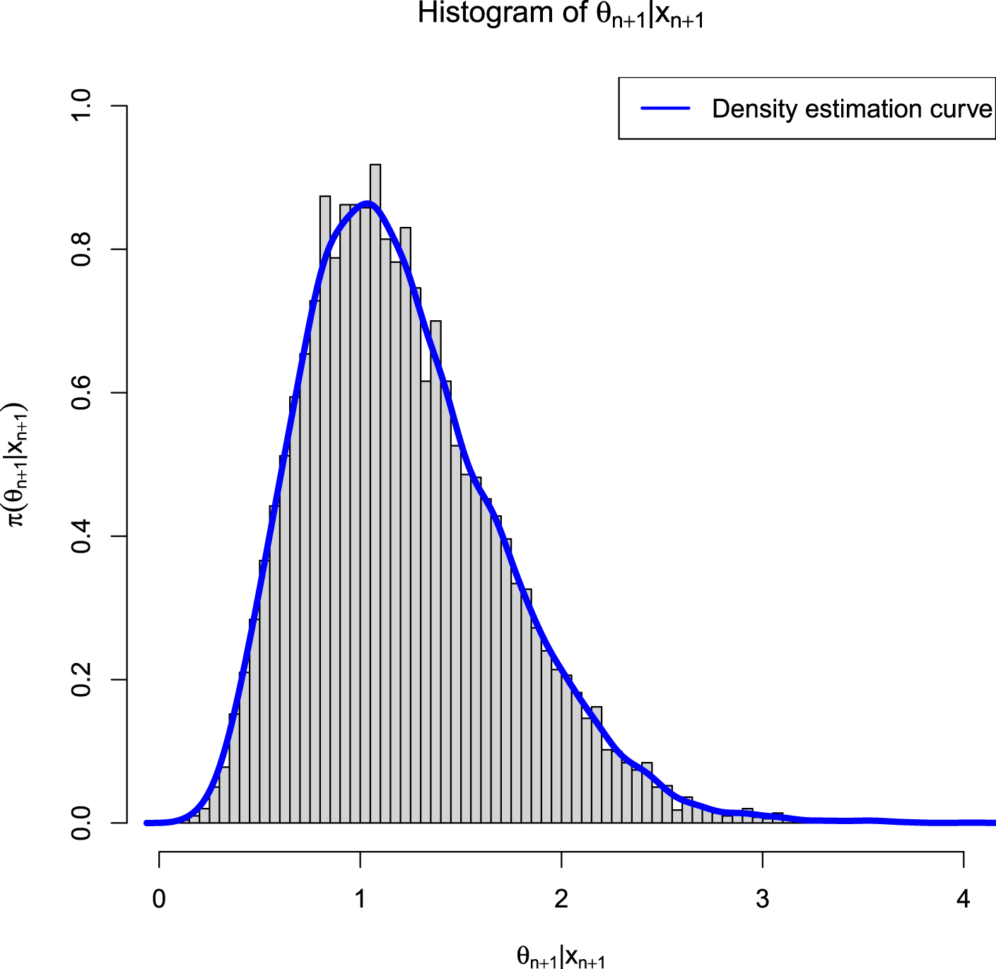
, , and . Then we set a seed number 1 in R software and draw from . After that, we draw from . Figure 3.1 shows the histogram of and the density estimation curve of . It is that we find to minimize the PESL. Numerical results show that
FIG. 3.1 — G-G: The histogram of  and the density estimation curve of
  .
.
and the density estimation curve of .
In figure 3.2, we fix  ,
,  , and
, and  , but allow
  to change from 1 to 10. From the figure, we see that the Bayes estimators and the PESLs are functions of
  . The numerical values of the Bayes estimators and the PESLs in figure 3.2 are displayed in table 3.1. We see from plot (a) or the first two lines of table 3.1 that the Bayes estimators are decreasing functions of
  , and
, and  are unanimously smaller than
  , and thus (3.6) is exemplified. Plot (b) or the last two lines of table 3.1 exhibit that the PESLs do not depend on
  , and
, and  are unanimously smaller than
  , and thus (3.9) is exemplified.
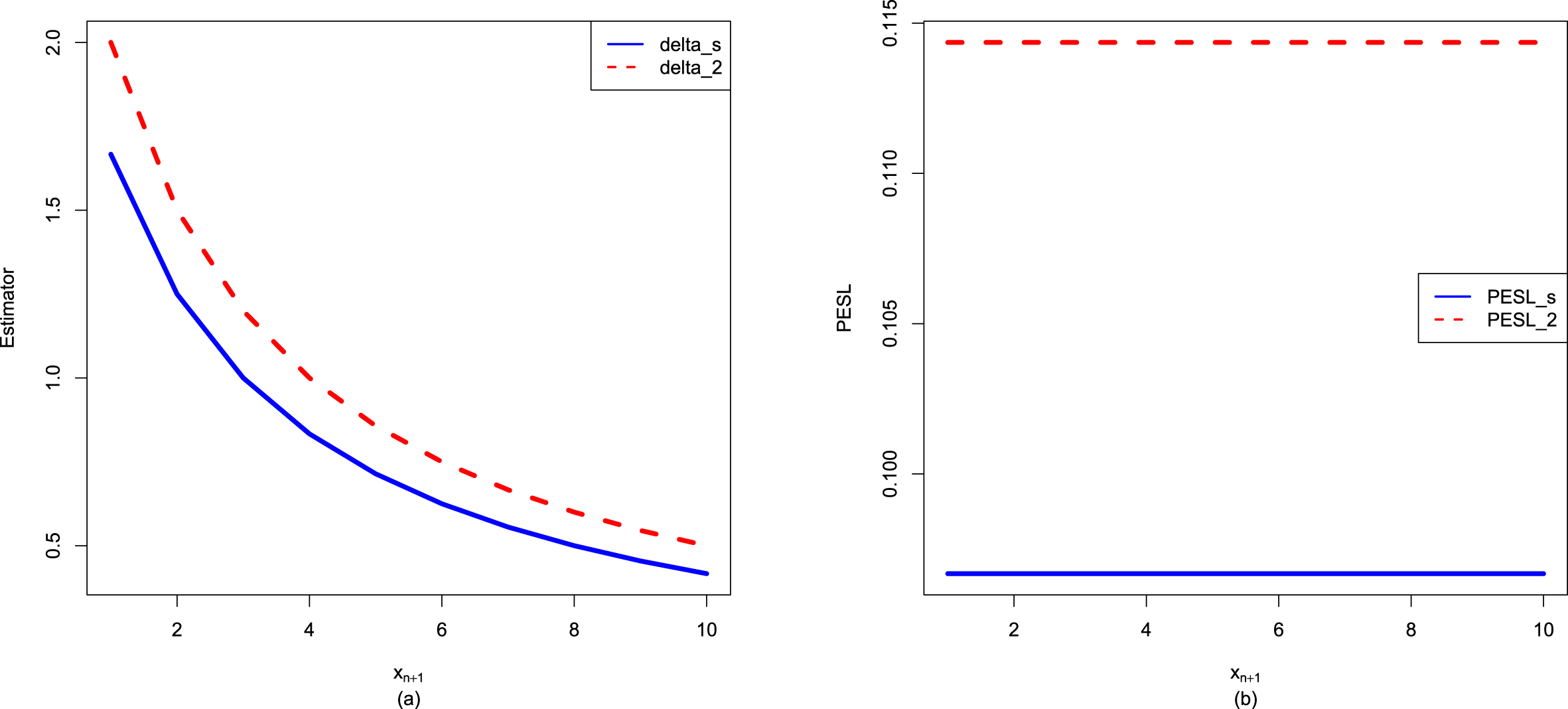
, , and , but allow to change from 1 to 10. From the figure, we see that the Bayes estimators and the PESLs are functions of . The numerical values of the Bayes estimators and the PESLs in figure 3.2 are displayed in table 3.1. We see from plot (a) or the first two lines of table 3.1 that the Bayes estimators are decreasing functions of , and are unanimously smaller than , and thus (3.6) is exemplified. Plot (b) or the last two lines of table 3.1 exhibit that the PESLs do not depend on , and are unanimously smaller than , and thus (3.9) is exemplified.
FIG. 3.2 — G-G: The Bayes estimators and the PESLs as functions of  . (a) Bayes estimators. (b) PESLs.
. (a) Bayes estimators. (b) PESLs.
TAB. 3.1 — G-G: The numerical values of the Bayes estimators and the PESLs in figure 3.2:  changes.
changes.
 |
1 | 2 | 3 | 4 | 5 | 6 | 7 | 8 | 9 | 10 |
 |
1.6667 | 1.2500 | 1.0000 | 0.8333 | 0.7143 | 0.6250 | 0.5556 | 0.5000 | 0.4545 | 0.4167 |
 |
2.0000 | 1.5000 | 1.2000 | 1.0000 | 0.8571 | 0.7500 | 0.6667 | 0.6000 | 0.5455 | 0.5000 |
 |
0.0967 | 0.0967 | 0.0967 | 0.0967 | 0.0967 | 0.0967 | 0.0967 | 0.0967 | 0.0967 | 0.0967 |
 |
0.1144 | 0.1144 | 0.1144 | 0.1144 | 0.1144 | 0.1144 | 0.1144 | 0.1144 | 0.1144 | 0.1144 |
Now we allow one of the three parameters  ,
,  , and
, and  to change, holding other parameters fixed. Moreover, we also assume that the datum
  is fixed, as is the case for the real data. Figure 3.3 shows the Bayes estimators and the PESLs as functions of
  ,
,  , and
, and  . We see from the left plots of the figure that the Bayes estimators depend on
  ,
,  , and
, and  , and (3.6) is exemplified. Moreover, the Bayes estimators are increasing functions of
  and
and  , and they are decreasing functions of
  . The right plots of the figure exhibit that the PESLs depend on
  and
and  , but not on
  , and (3.9) is exemplified. In addition, the PESLs are decreasing functions of
  and
and  . Furthermore, tables 3.2–3.4 display the numerical values of the Bayes estimators and the PESLs in figure 3.3. In summary, the results of figure 3.3 and tables 3.2–3.4 exemplify the theoretical studies of (3.6) and (3.9).
, , and to change, holding other parameters fixed. Moreover, we also assume that the datum is fixed, as is the case for the real data. Figure 3.3 shows the Bayes estimators and the PESLs as functions of , , and . We see from the left plots of the figure that the Bayes estimators depend on , , and , and (3.6) is exemplified. Moreover, the Bayes estimators are increasing functions of and , and they are decreasing functions of . The right plots of the figure exhibit that the PESLs depend on and , but not on , and (3.9) is exemplified. In addition, the PESLs are decreasing functions of and . Furthermore, tables 3.2–3.4 display the numerical values of the Bayes estimators and the PESLs in figure 3.3. In summary, the results of figure 3.3 and tables 3.2–3.4 exemplify the theoretical studies of (3.6) and (3.9).
TAB. 3.2 — G-G: The numerical values of the Bayes estimators and the PESLs in figure 3.3:  changes.
changes.
 |
4 | 5 | 6 | 7 | 8 | 9 | 10 | 11 | 12 | 13 |
 |
2.0700 | 2.4840 | 2.8980 | 3.3120 | 3.7260 | 4.1400 | 4.5540 | 4.9681 | 5.3821 | 5.7961 |
 |
2.4840 | 2.8980 | 3.3120 | 3.7260 | 4.1400 | 4.5540 | 4.9681 | 5.3821 | 5.7961 | 6.2101 |
 |
0.0967 | 0.0810 | 0.0697 | 0.0612 | 0.0545 | 0.0492 | 0.0448 | 0.0411 | 0.0380 | 0.0353 |
 |
0.1144 | 0.0935 | 0.0791 | 0.0684 | 0.0603 | 0.0539 | 0.0487 | 0.0444 | 0.0408 | 0.0377 |
Since the Bayes estimators  and
and  and the PESLs
  and
and  depend on
  and
and  , where
  and
and  , we can plot the surfaces of the Bayes estimators and the PESLs on the domain
  via the R function persp3d() in the R package rgl (see Sun et al. (2021); Zhang et al. (2017, 2019b); Adler et al. (2017)). We remark that the R function persp() in the R package graphics can not add another surface to the existing surface, but persp3d() can. Moreover, persp3d() allows one to rotate the perspective plots of the surface according to one’s wishes. Figure 3.4 plots the surfaces of the Bayes estimators and the PESLs, and the surfaces of the differences of the Bayes estimators and the PESLs. The domain for
  is
is  for all the plots. a is for
  and b is for
  in the axes of all the plots. The red surface is for
  and the blue surface is for
  in the upper two plots. From the left two plots of the figure, we see that
  for all
  on
on  . From the right two plots of the figure, we see that
  for all
  on
on  . The results of the figure exemplify the theoretical studies of (3.6) and (3.9).
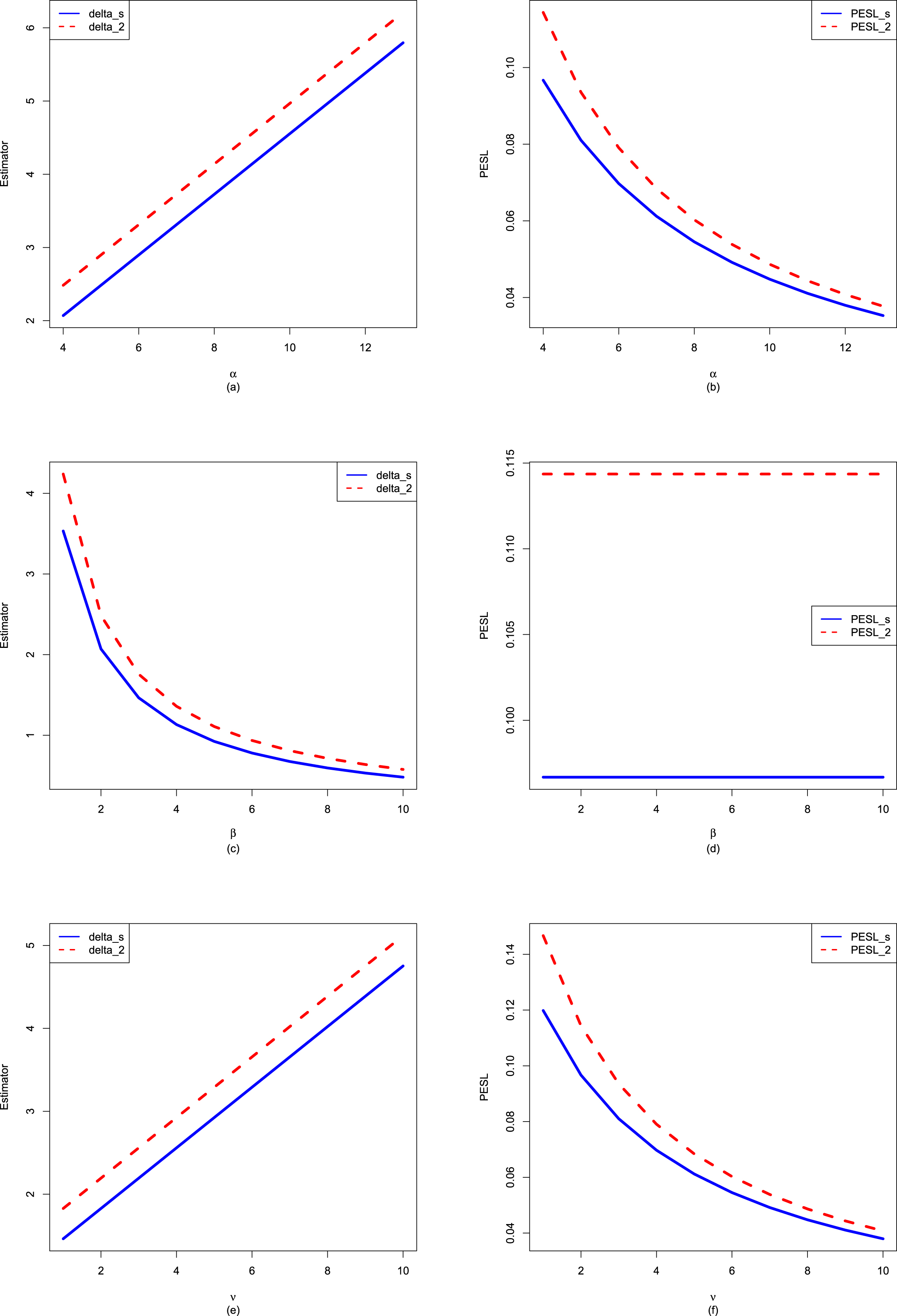
and and the PESLs and depend on and , where and , we can plot the surfaces of the Bayes estimators and the PESLs on the domain via the R function persp3d() in the R package rgl (see Sun et al. (2021); Zhang et al. (2017, 2019b); Adler et al. (2017)). We remark that the R function persp() in the R package graphics can not add another surface to the existing surface, but persp3d() can. Moreover, persp3d() allows one to rotate the perspective plots of the surface according to one’s wishes. Figure 3.4 plots the surfaces of the Bayes estimators and the PESLs, and the surfaces of the differences of the Bayes estimators and the PESLs. The domain for is for all the plots. a is for and b is for in the axes of all the plots. The red surface is for and the blue surface is for in the upper two plots. From the left two plots of the figure, we see that for all on . From the right two plots of the figure, we see that for all on . The results of the figure exemplify the theoretical studies of (3.6) and (3.9).
FIG. 3.3 — G-G: The Bayes estimators and the PESLs as functions of  ,
,  , and
, and  . (a) Bayes estimators vs.
  . (b) PESLs vs.
  . (c) Bayes estimators vs.
  . (d) PESLs vs.
  . (e) Bayes estimators vs.
  . (f) PESLs vs.
  .
.
, , and . (a) Bayes estimators vs. . (b) PESLs vs. . (c) Bayes estimators vs. . (d) PESLs vs. . (e) Bayes estimators vs. . (f) PESLs vs. .
TAB. 3.3 — G-G: The numerical values of the Bayes estimators and the PESLs in figure 3.3:  changes.
changes.
 |
1 | 2 | 3 | 4 | 5 | 6 | 7 | 8 | 9 | 10 |
 |
3.5325 | 2.0700 | 1.4639 | 1.1324 | 0.9233 | 0.7794 | 0.6743 | 0.5941 | 0.5310 | 0.4801 |
 |
4.2390 | 2.4840 | 1.7567 | 1.3589 | 1.1079 | 0.9352 | 0.8091 | 0.7130 | 0.6373 | 0.5761 |
 |
0.0967 | 0.0967 | 0.0967 | 0.0967 | 0.0967 | 0.0967 | 0.0967 | 0.0967 | 0.0967 | 0.0967 |
 |
0.1144 | 0.1144 | 0.1144 | 0.1144 | 0.1144 | 0.1144 | 0.1144 | 0.1144 | 0.1144 | 0.1144 |
TAB. 3.4 — G-G: The numerical values of the Bayes estimators and the PESLs in figure 3.3:  changes.
changes.
 |
1 | 2 | 3 | 4 | 5 | 6 | 7 | 8 | 9 | 10 |
 |
1.4624 | 1.8279 | 2.1935 | 2.5591 | 2.9247 | 3.2903 | 3.6559 | 4.0215 | 4.3871 | 4.7527 |
 |
1.8279 | 2.1935 | 2.5591 | 2.9247 | 3.2903 | 3.6559 | 4.0215 | 4.3871 | 4.7527 | 5.1182 |
 |
0.1198 | 0.0967 | 0.0810 | 0.0697 | 0.0612 | 0.0545 | 0.0492 | 0.0448 | 0.0411 | 0.0380 |
 |
0.1467 | 0.1144 | 0.0935 | 0.0791 | 0.0684 | 0.0603 | 0.0539 | 0.0487 | 0.0444 | 0.0408 |
3.3.2 Consistencies of the Moment Estimators and the MLEs
In this subsection, similar to subsection 1.8.1, we will numerically exemplify that the moment estimators and the MLEs are consistent estimators of the hyperparameters  ,
,  , and
, and  of the hierarchical gamma and gamma model (3.1). The motivation of this subsection is that in Theorems 3.2 and 3.3, we have theoretically shown that the moment estimators and the MLEs are consistent estimators of the hyperparameters. Note that only
  are used in this subsection.
, , and of the hierarchical gamma and gamma model (3.1). The motivation of this subsection is that in Theorems 3.2 and 3.3, we have theoretically shown that the moment estimators and the MLEs are consistent estimators of the hyperparameters. Note that only are used in this subsection.
The frequencies of the moment estimators ( ,
,  , and
, and  ) and the MLEs (
 ,
,  , and
, and  ) of the hyperparameters (
 ,
,  , and
, and  ) as
) as  varies for
  and
and  , 0.5, and 0.1 are reported in table 3.5. From the table, we observe the following facts.
, , and ) and the MLEs (, , and ) of the hyperparameters (, , and ) as varies for and , 0.5, and 0.1 are reported in table 3.5. From the table, we observe the following facts.
1. Given  , 0.5, or 0.1, the frequencies of the estimators (
 ,
,  ,
,  , or
, or  ,
,  ) tend to 0 as
  increases to infinity, which means that the moment estimators and the MLEs are consistent estimators of the hyperparameters. For
  , the frequencies of the estimators are still very large. However, we observe the tendencies of declining to 0 as
  increases to infinity.
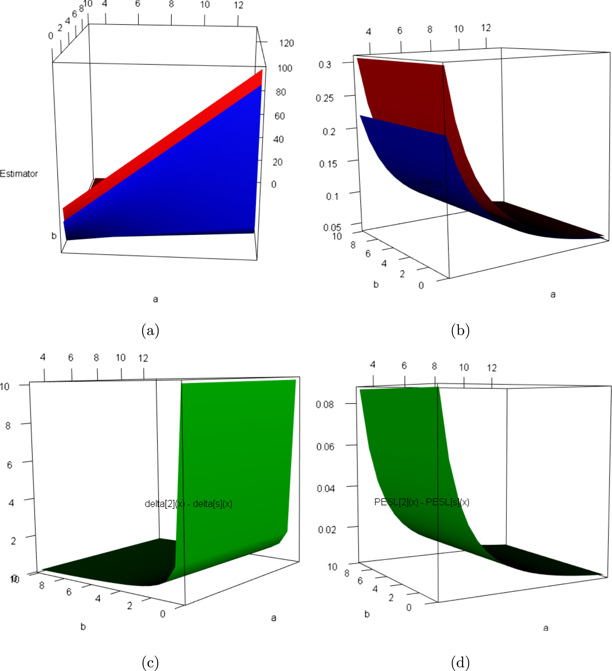
, 0.5, or 0.1, the frequencies of the estimators (, , , or , ) tend to 0 as increases to infinity, which means that the moment estimators and the MLEs are consistent estimators of the hyperparameters. For , the frequencies of the estimators are still very large. However, we observe the tendencies of declining to 0 as increases to infinity.
FIG. 3.4 — G-G: (a) The Bayes estimators as functions of  and
and  . (b) The PESLs as functions of
  and
and  . (c) The surface of
  which is positive for all
  on
on  . (d) The surface of
  which is also positive for all
  on
on  .
.
and . (b) The PESLs as functions of and . (c) The surface of which is positive for all on . (d) The surface of which is also positive for all on .
2. Comparing the frequencies corresponding to  , 0.5, and 0.1, we observe that as
  gets smaller, the frequencies tend to be larger, since the constraints

, 0.5, and 0.1, we observe that as gets smaller, the frequencies tend to be larger, since the constraints
are easier to meet.
3. Comparing the moment estimators and the MLEs of the hyperparameters  ,
,  , and
, and  , we see that the frequencies of the MLEs are smaller than those of the moment estimators, which means that the MLEs are better than the moment estimators when estimating the hyperparameters in terms of consistency.
, , and , we see that the frequencies of the MLEs are smaller than those of the moment estimators, which means that the MLEs are better than the moment estimators when estimating the hyperparameters in terms of consistency.
3.3.3 Goodness-of-Fit of the Model: KS Test
In this subsection, similar to subsection 1.8.2, we will calculate the goodness-of-fit of the hierarchical gamma and gamma model (3.1) to the simulated data. The motivation of this subsection is that we want to check whether the marginal distribution of the hierarchical gamma and gamma model (3.1) fits the simulated data well. Note that only  are used in this subsection.
are used in this subsection.
In our problem, the null hypothesis specifies that
 where
where  is the marginal distribution of the hierarchical gamma and gamma model (3.1). The marginal density of the
  distribution is given by (3.3), which is obviously one-dimensional continuous. Hence, the KS test can be utilized as a measure of the goodness-of-fit.
is the marginal distribution of the hierarchical gamma and gamma model (3.1). The marginal density of the distribution is given by (3.3), which is obviously one-dimensional continuous. Hence, the KS test can be utilized as a measure of the goodness-of-fit.
The results of the KS test goodness-of-fit of the model (3.1) to the simulated data are reported in table 3.6. Note that the data are simulated according to the hierarchical gamma and gamma model (3.1) with  ,
,  , and
, and  . In the table, the hyperparameters
  ,
,  , and
, and  are estimated by three methods. The first method is the oracle method, in that we know the hyperparameters
  ,
,  , and
, and  . The second method is the moment method, in that the hyperparameters
  ,
,  , and
, and  are estimated by their moment estimators (see Theorem 3.2). The third method is the MLE method, in that the hyperparameters
  ,
,  , and
, and  are estimated by their MLEs (see Theorem 3.3). In the table, the sample size is
  , and the number of simulations is
  .
.
, , and . In the table, the hyperparameters , , and are estimated by three methods. The first method is the oracle method, in that we know the hyperparameters , , and . The second method is the moment method, in that the hyperparameters , , and are estimated by their moment estimators (see Theorem 3.2). The third method is the MLE method, in that the hyperparameters , , and are estimated by their MLEs (see Theorem 3.3). In the table, the sample size is , and the number of simulations is .
TAB. 3.5 — G-G: The frequencies of the moment estimators and the MLEs of the hyperparameters as  varies for
  and
and  , 0.5, and 0.1.
varies for and , 0.5, and 0.1.
| Moment estimators | MLEs | ||||||
 |
 |
 |
 |
 |
 |
 |
|
 |
1e4 | 0.27 | 0.56 | 0.01 | 0 | 0.01 | 0.01 |
| 2e4 | 0.21 | 0.46 | 0 | 0 | 0 | 0 | |
| 4e4 | 0.11 | 0.32 | 0 | 0 | 0 | 0 | |
| 8e4 | 0.04 | 0.21 | 0 | 0 | 0 | 0 | |
 |
1e4 | 0.70 | 0.78 | 0.15 | 0.04 | 0.04 | 0.02 |
| 2e4 | 0.63 | 0.75 | 0.04 | 0 | 0.01 | 0 | |
| 4e4 | 0.50 | 0.69 | 0.03 | 0.01 | 0.03 | 0.01 | |
| 8e4 | 0.44 | 0.60 | 0.03 | 0.01 | 0.01 | 0 | |
 |
1e4 | 0.95 | 0.99 | 0.92 | 0.60 | 0.55 | 0.07 |
| 2e4 | 0.92 | 0.93 | 0.91 | 0.44 | 0.36 | 0.01 | |
| 4e4 | 0.93 | 0.96 | 0.93 | 0.27 | 0.19 | 0.05 | |
| 8e4 | 0.91 | 0.93 | 0.90 | 0.13 | 0.08 | 0.01 | |
From table 3.6, we observe the following facts.
1. The  values for the three methods are respectively given by 0.2674, 0.0292, and 0.0088, which means that the MLE method is the best method, the moment method is the second-best method, and the oracle method is the worst method. A possible explanation for this phenomenon is that in (1.23), the empirical cdf
  is based on data, and the population cdfs
  for the MLE method and the moment method are also based on data, while the population cdf
  for the oracle method is not based on data.
values for the three methods are respectively given by 0.2674, 0.0292, and 0.0088, which means that the MLE method is the best method, the moment method is the second-best method, and the oracle method is the worst method. A possible explanation for this phenomenon is that in (1.23), the empirical cdf is based on data, and the population cdfs for the MLE method and the moment method are also based on data, while the population cdf for the oracle method is not based on data.
2. The  values for the three methods are respectively given by 0.0161, 0.0679, and 0.7956, which also means that the MLE method ranks first, the moment method ranks second, and the oracle method ranks third. The possible explanation for this phenomenon is described in the previous paragraph.
values for the three methods are respectively given by 0.0161, 0.0679, and 0.7956, which also means that the MLE method ranks first, the moment method ranks second, and the oracle method ranks third. The possible explanation for this phenomenon is described in the previous paragraph.
3. The  values for the three methods are respectively given by 0.01, 0.06, and 0.93. The
  value for the MLE method accounts for nearly all of the
  simulations. The order of preference for the three methods is the MLE method, the moment method, and the oracle method.
values for the three methods are respectively given by 0.01, 0.06, and 0.93. The value for the MLE method accounts for nearly all of the simulations. The order of preference for the three methods is the MLE method, the moment method, and the oracle method.
4. The  values for the three methods are respectively given by 0.02, 0.07, and 0.91. The
  value for the MLE method accounts for nearly all of the
  simulations. The order of preference for the three methods is the MLE method, the moment method, and the oracle method.
values for the three methods are respectively given by 0.02, 0.07, and 0.91. The value for the MLE method accounts for nearly all of the simulations. The order of preference for the three methods is the MLE method, the moment method, and the oracle method.
5. The  values for the three methods are respectively given by 0.04, 0.20, and 0.95. Once again, the order of preference for the three methods is the MLE method, the moment method, and the oracle method. The
  value for the MLE method is over
  , which means that the MLE method has good performance in terms of goodness-of-fit.
values for the three methods are respectively given by 0.04, 0.20, and 0.95. Once again, the order of preference for the three methods is the MLE method, the moment method, and the oracle method. The value for the MLE method is over , which means that the MLE method has good performance in terms of goodness-of-fit.
6. In summary, for the five indices ( ,
,  ,
,  ,
,  ,
,  ), the order of preference for the three methods is the MLE method, the moment method, and the oracle method. Comparing the moment method and the MLE method, we find that the MLE method has a better performance than the moment method in terms of all five indices.
, , , , ), the order of preference for the three methods is the MLE method, the moment method, and the oracle method. Comparing the moment method and the MLE method, we find that the MLE method has a better performance than the moment method in terms of all five indices.
TAB. 3.6 — G-G: The results of the KS test goodness-of-fit of the model (3.1) to the simulated data.
 |
 |
 |
|
 |
0.2674 | 0.0292 | 0.0088 |
 |
0.0161 | 0.0679 | 0.7956 |
 |
0.01 | 0.06 | 0.93 |
 % % |
0.02 | 0.07 | 0.91 |
 % % |
0.04 | 0.20 | 0.95 |
The boxplots of the  values and the p-values for the three methods are displayed in figure 3.5. From the figure, we observe the following facts.
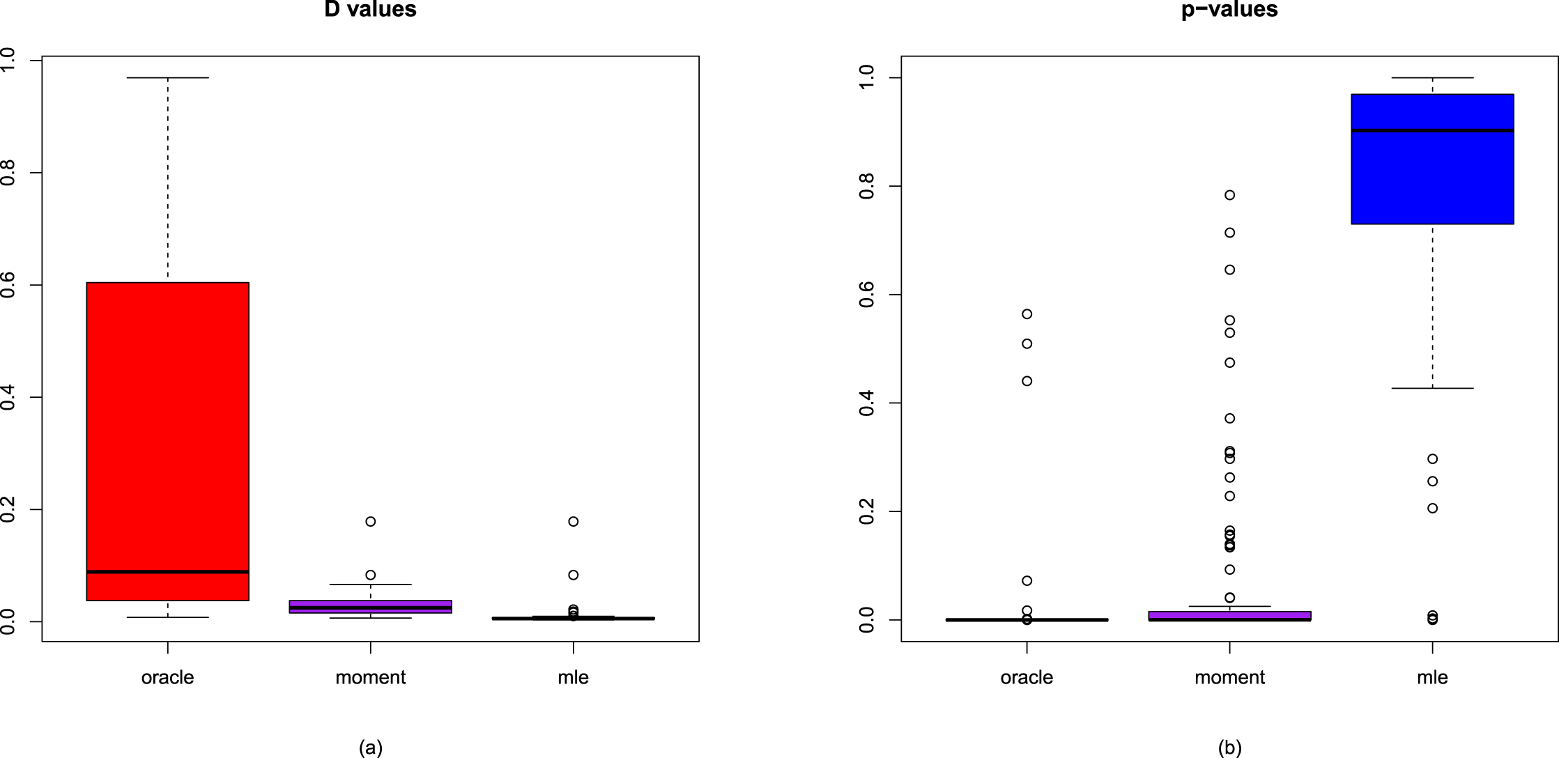
values and the p-values for the three methods are displayed in figure 3.5. From the figure, we observe the following facts.
1. The  values of the oracle method are significantly larger than those of the other two methods. Since for the
  value, the smaller the better, the order of preference for the three methods is the MLE method, the moment method, and the oracle method.
values of the oracle method are significantly larger than those of the other two methods. Since for the value, the smaller the better, the order of preference for the three methods is the MLE method, the moment method, and the oracle method.
2. The p-values of the MLE method are significantly larger than those of the other two methods. Since for the p-value, the larger the better, the order of preference for the three methods is the MLE method, the moment method, and the oracle method.
3. Small  values correspond to large p-values, and large
  values correspond to small p-values.
values correspond to large p-values, and large values correspond to small p-values.
4. The MLE method has a better performance than the moment method in terms of the  values and the p-values.
values and the p-values.
FIG. 3.5 — G-G: The boxplots of the  values and the p-values for the three methods. (a)
  values. (b) p-values.
values and the p-values for the three methods. (a) values. (b) p-values.
3.3.4 Numerical Comparisons of the Bayes Estimators and the PESLs of Three Methods
In this subsection, we will numerically compare the Bayes estimators and the PESLs of the three methods (the oracle method, the moment method, and the MLE method). The motivation of this subsection is that the theoretical comparisons of the Bayes estimators and the PESLs of the three methods can be found in subsection 3.2.3. Note that the full data  are used in this subsection.
are used in this subsection.
Note that the data are simulated according to the hierarchical gamma and gamma model (3.1) with hyperparameters  ,
,  , and
, and  . Moreover, the oracle method knows the hyperparameters
  ,
,  , and
, and  in simulations.
, , and . Moreover, the oracle method knows the hyperparameters , , and in simulations.
Comparisons of the Bayes estimators and the PESLs of the three methods for sample size  and number of simulations
  are displayed in figure 3.6. From the figure, we observe the following facts.
and number of simulations are displayed in figure 3.6. From the figure, we observe the following facts.
1. Plot (a): For the Bayes estimators of  under Stein’s loss function
 , the MLE method is slightly closer to the oracle method than the moment method.
under Stein’s loss function , the MLE method is slightly closer to the oracle method than the moment method.
2. Plot (b): For the Bayes estimators of  under the squared error loss function
 , the MLE method is also slightly closer to the oracle method than the moment method.
under the squared error loss function , the MLE method is also slightly closer to the oracle method than the moment method.
3. Plot (c): For the PESLs 
 , the MLE method is much closer to the oracle method than the moment method.
, the MLE method is much closer to the oracle method than the moment method.
4. Plot (d): For the PESLs 
 , the MLE method is also much closer to the oracle method than the moment method.
, the MLE method is also much closer to the oracle method than the moment method.
5. All four plots indicate that the MLE method is better than the moment method, as the Bayes estimators and the PESLs of the MLE method are closer to those of the oracle method than those of the moment method.
The boxplots of the absolute errors from the oracle method by the moment method and the MLE method for sample size  and number of simulations
  are displayed in figure 3.7. All four plots indicate that the MLE method is better than the moment method, as the absolute errors from the oracle method of the Bayes estimators and the PESLs by the MLE method are much smaller than those by the moment method.
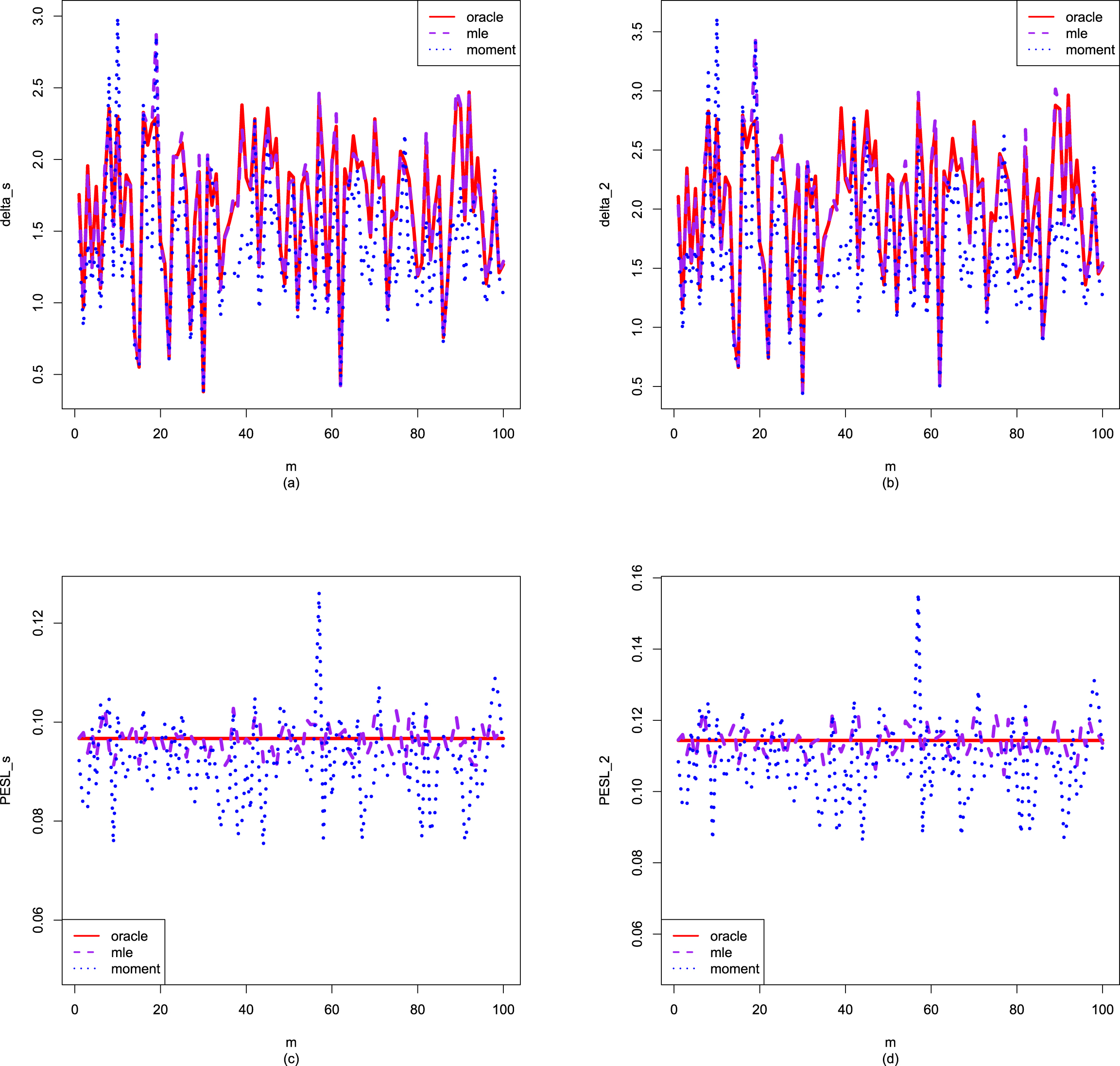
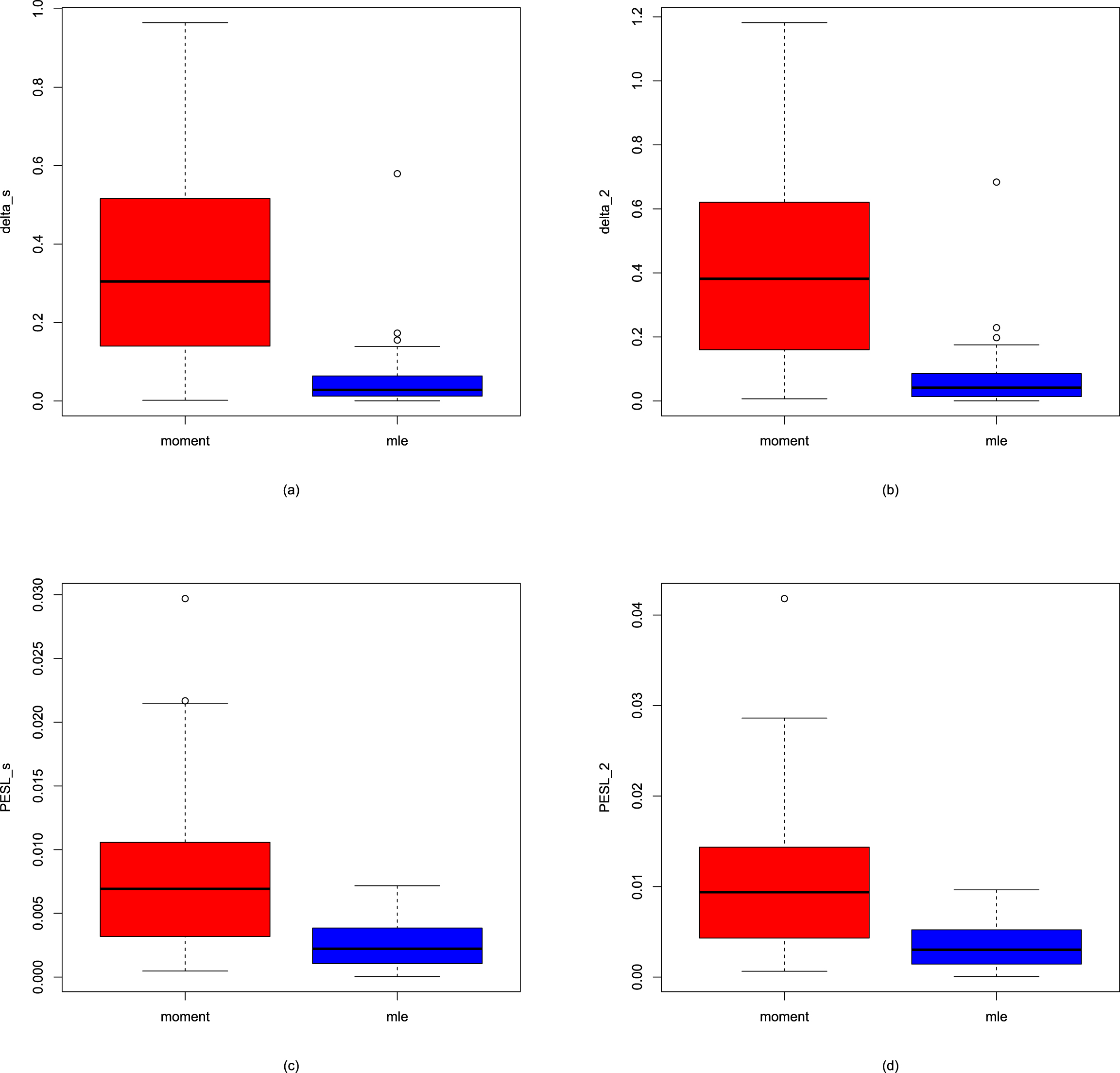
and number of simulations are displayed in figure 3.7. All four plots indicate that the MLE method is better than the moment method, as the absolute errors from the oracle method of the Bayes estimators and the PESLs by the MLE method are much smaller than those by the moment method.
FIG. 3.6 — G-G: Comparisons of the Bayes estimators and the PESLs of the three methods for sample size  and number of simulations
  . (a)
. (a) 
 . (b)
. (b) 
 . (c)
. (c) 
 . (d)
. (d) 
 .
.
and number of simulations . (a) . (b) . (c) . (d) .
FIG. 3.7 — G-G: The boxplots of the absolute errors from the oracle method by the moment method and the MLE method for sample size  and number of simulations
  . (a) Absolute errors for
  . (b) Absolute errors for
  . (c) Absolute errors for
  . (d) Absolute errors for
  .
.
and number of simulations . (a) Absolute errors for . (b) Absolute errors for . (c) Absolute errors for . (d) Absolute errors for .
The averages and proportions of the absolute errors from the oracle method by the moment method and the MLE method for the Bayes estimators and the PESLs are summarized in table 3.7. See subsection 1.8.3 for details. From the table, we observe that the averages of the absolute errors from the oracle method by the MLE method are much smaller than those by the moment method. Moreover, the proportions of the absolute errors from the oracle method by the MLE method are much larger than those by the moment method. In summary, the table illustrates that the MLE method is better than the moment method in terms of the averages and proportions of the absolute errors from the oracle method.
TAB. 3.7 — G-G: The averages and proportions of the absolute errors from the oracle method by the moment method and the MLE method for the Bayes estimators and the PESLs.
| Averages | Proportions | |||
| Moment | MLE | Moment | MLE | |
 |
0.3332 | 0.0485 | 0.06 | 0.94 |
 |
0.4136 | 0.0621 | 0.06 | 0.94 |
 |
0.0079 | 0.0025 | 0.15 | 0.85 |
 |
0.0107 | 0.0034 | 0.15 | 0.85 |
3.3.5 Marginal Densities for Various Hyperparameters
In this subsection, we will plot the marginal densities of the hierarchical gamma and gamma model (3.1) for various hyperparameters  ,
,  , and
, and  . The motivation of this subsection is that we want to know what kind of data can be modeled by the hierarchical gamma and gamma model (3.1). Note that the marginal density of
  is given by (3.3) specified by three hyperparameters
  ,
,  , and
, and  . We will explore how the marginal densities change around the marginal density with hyperparameters specified by
  ,
,  , and
, and  . Other numerical values of the hyperparameters can also be specified.
, , and . The motivation of this subsection is that we want to know what kind of data can be modeled by the hierarchical gamma and gamma model (3.1). Note that the marginal density of is given by (3.3) specified by three hyperparameters , , and . We will explore how the marginal densities change around the marginal density with hyperparameters specified by , , and . Other numerical values of the hyperparameters can also be specified.
Figure 3.8 plots the marginal densities for varied  , holding
  and
and  fixed. From the figure, we see that as
  increases, the peak value of the curve increases. In other words, the variance of the marginal density decreases, as
 (3.16)
is a decreasing function of
(3.16)
is a decreasing function of  . Moreover, all the marginal densities are right-skewed.
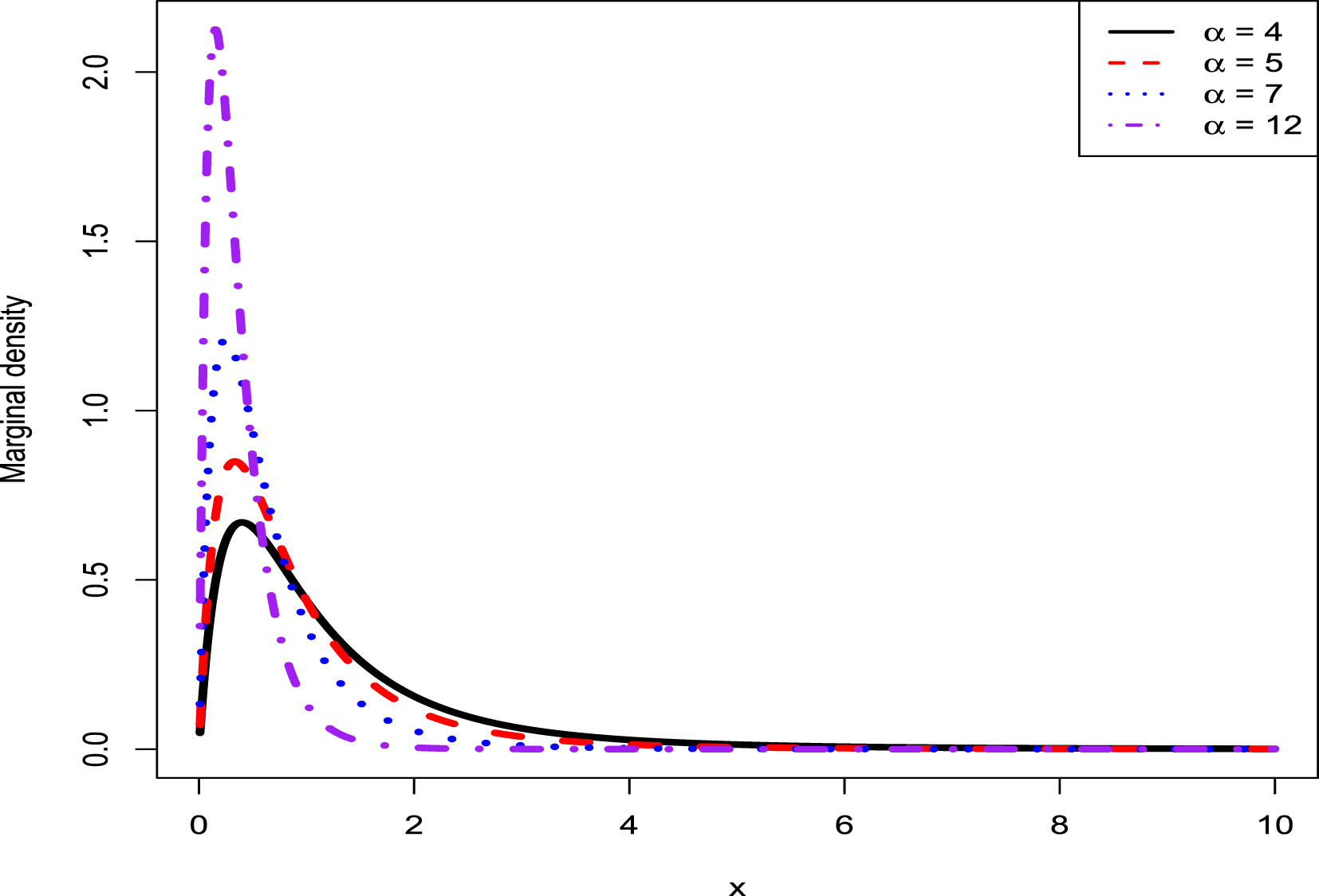
, holding and fixed. From the figure, we see that as increases, the peak value of the curve increases. In other words, the variance of the marginal density decreases, as
(3.16)
. Moreover, all the marginal densities are right-skewed.
FIG. 3.8 — G-G: The marginal densities for varied  , holding
  and
and  fixed.
, holding and fixed.
Figure 3.9 plots the marginal densities for varied  , holding
  and
and  fixed. From the figure, we see that as
  increases, the peak value of the curve decreases. In other words, the variance of the marginal density increases, as (3.16) is an increasing function of
  . Moreover, all the marginal densities are also right-skewed.
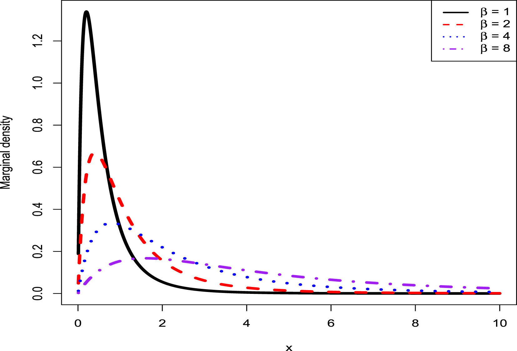
, holding and fixed. From the figure, we see that as increases, the peak value of the curve decreases. In other words, the variance of the marginal density increases, as (3.16) is an increasing function of . Moreover, all the marginal densities are also right-skewed.
FIG. 3.9 — G-G: The marginal densities for varied  , holding
  and
and  fixed.
, holding and fixed.
Figure 3.10 plots the marginal densities for varied  , holding
  and
and  fixed. From the figure, we see that as
  increases, the peak value of the curve decreases. In other words, the variance of the marginal density increases, as (3.16) is an increasing function of
  . Moreover, all the marginal densities are also right-skewed.
, holding and fixed. From the figure, we see that as increases, the peak value of the curve decreases. In other words, the variance of the marginal density increases, as (3.16) is an increasing function of . Moreover, all the marginal densities are also right-skewed.
3.4 Conclusions and Discussions
For the hierarchical gamma and gamma model (3.1), we calculate the posterior density  and the marginal density
  in Theorem 3.1. Since
  is a rate parameter in (3.1), the Bayes estimator of
  under the squared error loss function is not appropriate. In contrast, we should choose Stein’s loss function because it penalizes gross overestimation and gross underestimation equally. After that, we calculate the Bayes estimators of
  ,
,  and
and  , and the PESLs of
  ,
,  and
and  .
.
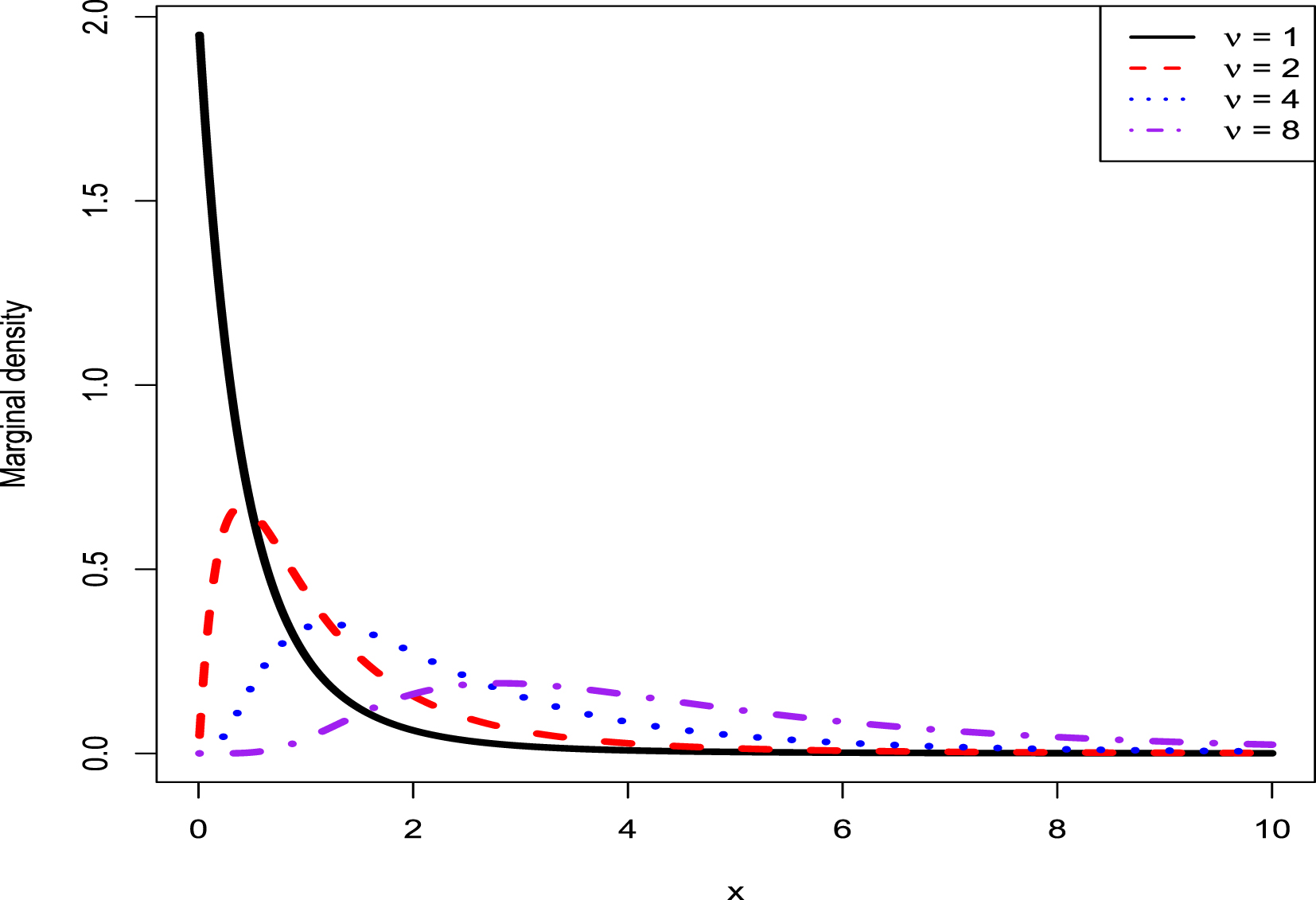
and the marginal density in Theorem 3.1. Since is a rate parameter in (3.1), the Bayes estimator of under the squared error loss function is not appropriate. In contrast, we should choose Stein’s loss function because it penalizes gross overestimation and gross underestimation equally. After that, we calculate the Bayes estimators of , and , and the PESLs of , and .
FIG. 3.10 — G-G: The marginal densities for varied  , holding
  and
and  fixed.
, holding and fixed.
In order to calculate the empirical Bayes estimator of the rate parameter  , we must calculate the estimators of the hyperparameters of model (3.1). The estimators of the hyperparameters of model (3.1) by the moment method and their consistencies are summarized in Theorem 3.2. Moreover, the estimators of the hyperparameters of model (3.1) by the MLE method and their consistencies are summarized in Theorem 3.3. Finally, the empirical Bayes estimators of the rate parameter
  of the model (3.1) under Stein’s loss function by the moment method and the MLE method are summarized in Theorem 3.4.
, we must calculate the estimators of the hyperparameters of model (3.1). The estimators of the hyperparameters of model (3.1) by the moment method and their consistencies are summarized in Theorem 3.2. Moreover, the estimators of the hyperparameters of model (3.1) by the MLE method and their consistencies are summarized in Theorem 3.3. Finally, the empirical Bayes estimators of the rate parameter of the model (3.1) under Stein’s loss function by the moment method and the MLE method are summarized in Theorem 3.4.
Note that in Theorem 3.3, we only stated that the estimators of the hyperparameters of the model (3.1) by the MLE method  ,
,  , and
, and  are the solutions to the equations (3.13)–(3.15). We can exploit Newton’s method to solve the equations (3.13)–(3.15), and to numerically obtain the MLEs of
  ,
,  , and
, and  . However, we can not prove the existence and uniqueness of the solutions to our system. The interested readers who have such knowledge and skills are encouraged to solve this issue.
, , and are the solutions to the equations (3.13)–(3.15). We can exploit Newton’s method to solve the equations (3.13)–(3.15), and to numerically obtain the MLEs of , , and . However, we can not prove the existence and uniqueness of the solutions to our system. The interested readers who have such knowledge and skills are encouraged to solve this issue.
Numerical simulations illustrate that the moment estimators and the MLEs are consistent estimators of the hyperparameters, as reported in table 3.5. Moreover, table 3.6 indicates that the hierarchical gamma and gamma model (3.1) fits the simulated data well in terms of the KS test goodness-of-fit by the moment method and the MLE method.
The plots of the marginal densities show that all the curves are right-skewed. Therefore, the hierarchical gamma and gamma model (3.1) could potentially be used to fit right-skewed data, not left-skewed data.
It is common to assume that a positive parameter follows a gamma distribution or an inverse gamma distribution. Therefore, the hierarchical gamma and gamma model (3.1), as a more variable gamma distribution, could be used to model the positive parameter.
Now we present some future work. One may consider extending the hierarchical gamma and gamma model (3.1) to different types of non-conjugate priors for the rate parameter of the gamma distribution (see Berger et al. (2015); Berger (1985) and the references therein). In these situations, one may not obtain analytical solutions, then one should be able to derive the estimators numerically.
Chapter 4 The Empirical Bayes Estimators of the Mean Parameter of the Exponential Distribution with a Conjugate Inverse Gamma Prior under Stein’s Loss Function
A Bayes estimator for a mean parameter of an exponential distribution is calculated using Stein’s loss, which equally penalizes gross overestimation and underestimation. A corresponding PESL is also determined. Additionally, a Bayes estimator for a mean parameter is obtained under a squared error loss along with its corresponding PESL. Furthermore, two methods are used to derive empirical Bayes estimators for the mean parameter of the exponential distribution with an inverse gamma prior. Numerical simulations are conducted to illustrate five aspects. Finally, theoretical studies are illustrated using Static Fatigue 90% Stress Level data.
Acknowledgement. This chapter is derived in part from an article Li et al. (2025) published in Mathematics 19 May 2025 <Copyright by the authors>, available online: https://doi.org/10.3390/math13101658.
4.1 Introduction
In the hierarchical exponential and inverse gamma model (4.1), our parameter of interest is the mean  which is a positive parameter. Therefore, we will choose Stein’s loss function because it penalizes gross overestimation and gross underestimation equally.
which is a positive parameter. Therefore, we will choose Stein’s loss function because it penalizes gross overestimation and gross underestimation equally.
The rest of the chapter is organized as follows. In section 4.2, we will provide four theorems. More specifically, we calculate the posterior density and the marginal density for the hierarchical exponential and inverse gamma model (4.1) in Theorem 4.1. Moreover, the estimators of the hyperparameters of the model by the moment method and their consistencies are summarized in Theorem 4.2. Furthermore, the estimators of the hyperparameters of the model by the MLE method and their consistencies are summarized in Theorem 4.3. Finally, the empirical Bayes estimators of the parameter of the model under Stein’s loss function by the moment method and the MLE method are summarized in Theorem 4.4. In section 4.3, we will illustrate five aspects in the numerical simulations. First, we will numerically exemplify two inequalities of the Bayes estimators and the PESLs. Second, we will illustrate that the moment estimators and the MLEs are consistent estimators of the hyperparameters. Third, we will calculate the goodness-of-fit of the model to the simulated data. Fourth, we will numerically compare the Bayes estimators and the PESLs of the three methods. Finally, we will plot the marginal densities of the model for various hyperparameters. In section 4.4, we utilize the Static Fatigue 90% Stress Level data to illustrate the calculations of the empirical Bayes estimators of the mean parameter of the exponential distribution with a conjugate inverse gamma prior. Some conclusions and discussions are provided in section 4.5.
4.2 Theoretical Results
Suppose that we observe  from the hierarchical exponential and inverse gamma model:
 (4.1)
where
(4.1)
where  and
and  are hyperparameters to be estimated,
  is the unknown parameter of interest,
  is the exponential distribution with mean parameter
  , and
, and  is the inverse gamma distribution with shape parameter
  and scale parameter β. As described in Deely and Lindley (1981), the statistician observes data
  and wishes to make an inference about
  . Therefore,
  provides direct information about the parameter
  , while supplementary information
  is also available. The connection between the prime data
  and the supplementary information
  is provided by the common distributions
  and
and  . The pdfs of
  and
and  can be found in section 1.2.
from the hierarchical exponential and inverse gamma model:
(4.1)
and are hyperparameters to be estimated, is the unknown parameter of interest, is the exponential distribution with mean parameter , and is the inverse gamma distribution with shape parameter and scale parameter β. As described in Deely and Lindley (1981), the statistician observes data and wishes to make an inference about . Therefore, provides direct information about the parameter , while supplementary information is also available. The connection between the prime data and the supplementary information is provided by the common distributions and . The pdfs of and can be found in section 1.2.
There are two pdf forms for the exponential distribution. One form uses the mean (or scale)  as the parameter (see Casella and Berger (2002)), and
  with pdf
  , for
, for  and
and  . Another form utilizes the rate
  as the parameter (see Gelman et al. (2013); Mao and Tang (2012)), and
  with pdf
  , for
, for  and
and  . The two pdfs are the same with a relationship of the parameters
  .
.
as the parameter (see Casella and Berger (2002)), and with pdf , for and . Another form utilizes the rate as the parameter (see Gelman et al. (2013); Mao and Tang (2012)), and with pdf , for and . The two pdfs are the same with a relationship of the parameters .
The exponential-gamma model is assumed to generate observations  :
:
 (4.2)
(4.2)
:
(4.2)
Firstly, the exponential-inverse gamma model (4.1) and the exponential-gamma model (4.2) are equivalent in the sense of their marginal pdfs. For convenience, now let  ,
,  ,
,  ,
,  ,
,  , and
, and  be random variables having the corresponding distributions. For example,
  is a random variable having the
  distribution. It is easy to see that

, , , , , and be random variables having the corresponding distributions. For example, is a random variable having the distribution. It is easy to see that
Therefore, the two hierarchical models (4.1) and (4.2) are equivalent. It is straightforward to derive that the two marginal pdfs of the two hierarchical models are the same, and they are equal to

Since the two marginal pdfs are the same, the moment estimators (displayed in Theorem 4.2) and the MLEs (see Theorem 4.3) of the hyperparameters  and
and  for the two hierarchical models (4.1) and (4.2) are the same.
and for the two hierarchical models (4.1) and (4.2) are the same.
Another reason to use (4.1) is that it motivates us to consider 16 hierarchical models of the gamma and inverse gamma distributions (see Zhang and Zhang (2022)). It is easy to see that  is a conjugate prior for the
  distribution. Writing in the form of likelihood-prior, it is
  . Similarly, the
  is a conjugate prior for the
  distribution. Writing in the form of likelihood-prior, it is
  . The
. The  expression motivates us to consider
  ,
,  ,
,  , and
, and  as the likelihood, and
  ,
,  ,
,  , and
, and  as the prior, leading to 16 combinations of the likelihood-prior.
is a conjugate prior for the distribution. Writing in the form of likelihood-prior, it is . Similarly, the is a conjugate prior for the distribution. Writing in the form of likelihood-prior, it is . The expression motivates us to consider , , , and as the likelihood, and , , , and as the prior, leading to 16 combinations of the likelihood-prior.
4.2.1 The Bayes Estimators and the PESLs
The posterior distribution of  and the marginal density of
  of the hierarchical exponential and inverse gamma model (4.1) are summarized in the following theorem whose proof can be found in appendix A.9.
and the marginal density of of the hierarchical exponential and inverse gamma model (4.1) are summarized in the following theorem whose proof can be found in appendix A.9.
Theorem 4.1. For the hierarchical exponential and inverse gamma model (4.1), the posterior distribution of  is
is
 (4.3)
where
(4.3)
where
 (4.4)
(4.4)
is
(4.3)
(4.4)
Moreover, the marginal density of  is
is
 (4.5)
for
(4.5)
for  and
and  .
.
is
(4.5)
and .
Now, let us analytically calculate the Bayes estimators  and
and  , and the PESLs
  and
and  under the hierarchical exponential and inverse gamma model (4.1).
and , and the PESLs and under the hierarchical exponential and inverse gamma model (4.1).
From (4.3), we have

From (1.12), the Bayes estimator of  under Stein’s loss function, it is given by
 (4.6)
where
(4.6)
where  and
and  are given by (4.4). Moreover, from (1.13), the Bayes posterior estimator of
  under the usual squared error loss function, it is given by
 (4.7)
for
(4.7)
for  . It is easy to see that
 (4.8)
which exemplifies the theoretical study of (1.16).
(4.8)
which exemplifies the theoretical study of (1.16).
under Stein’s loss function, it is given by
(4.6)
and are given by (4.4). Moreover, from (1.13), the Bayes posterior estimator of under the usual squared error loss function, it is given by
(4.7)
. It is easy to see that
(4.8)
To analytically calculate the PESLs  and
and  , we need to analytically calculate
  . For the sake of simplicity, the *’s are dropped from
  and
and  . We have

 where
where
 is the digamma function.
and , we need to analytically calculate . For the sake of simplicity, the *’s are dropped from and . We have
Therefore, from (1.14) and (1.15), after some algebraic operations, the PESLs at  and
and  are respectively given by
 (4.9)
and
(4.9)
and
 (4.10)
for
(4.10)
for  . It is easy to show that
 (4.11)
which exemplifies the theoretical study of (1.17). It is worth noting that the PESLs
(4.11)
which exemplifies the theoretical study of (1.17). It is worth noting that the PESLs  and
and  depend only on
  , but not on
  . Therefore, the PESLs depend only on
  , but not on
  and
and  .
.
and are respectively given by
(4.9)
(4.10)
. It is easy to show that
(4.11)
and depend only on , but not on . Therefore, the PESLs depend only on , but not on and .
In the simulations section and the real data section, we will exemplify the two inequalities (4.8) and (4.11). Moreover, we will exemplify that the PESLs depend only on  , but not on
  and
and  .
.
, but not on and .
It is worth noting that the Bayes estimators and the PESLs in this subsection assume that the hyperparameters  and
and  are known. In other words, the Bayes estimators and the PESLs in this subsection are calculated by the oracle method, which will be further discussed in subsection 4.2.3.
and are known. In other words, the Bayes estimators and the PESLs in this subsection are calculated by the oracle method, which will be further discussed in subsection 4.2.3.
4.2.2 The Empirical Bayes Estimators of θn+1
To obtain the empirical Bayes estimators of  , we need to estimate the hyperparameters from the supplementary information
  . There are two common methods to estimate the hyperparameters, that is, the moment method and the MLE method.
, we need to estimate the hyperparameters from the supplementary information . There are two common methods to estimate the hyperparameters, that is, the moment method and the MLE method.
The estimators of the hyperparameters of the model (4.1) by the moment method  and
and  , and their consistencies are summarized in the following theorem whose proof can be found in appendix A.10.
and , and their consistencies are summarized in the following theorem whose proof can be found in appendix A.10.
Theorem 4.2. The estimators of the hyperparameters of the model (4.1) by the moment method are
 (4.12)
 (4.13)
where
(4.13)
where  ,
,  , is the sample
  th moment of
  . Moreover, the moment estimators are consistent estimators of the hyperparameters.
(4.12)
(4.13)
, , is the sample th moment of . Moreover, the moment estimators are consistent estimators of the hyperparameters.
The estimators of the hyperparameters of the model (4.1) by the MLE method  and
and  , and their consistencies are summarized in the following theorem whose proof can be found in appendix A.11.
and , and their consistencies are summarized in the following theorem whose proof can be found in appendix A.11.
Theorem 4.3. The estimators of the hyperparameters of the model (4.1) by the MLE method  and
and  are the solutions to the following equations:
 (4.14)
 (4.15)
and are the solutions to the following equations:
(4.14)
(4.15)
Moreover, the MLEs are consistent estimators of the hyperparameters.
The analytical calculations of the MLEs of  and
and  by solving the equations (4.14) and (4.15) are impossible, and thus we have to resort to numerical solutions. We can exploit Newton’s method to solve the equations (4.14) and (4.15) and to obtain the MLEs of
  and
and  . Note that the MLEs of
  and
and  are very sensitive to the initial estimators, and the moment estimators are usually proved to be good initial estimators.
and by solving the equations (4.14) and (4.15) are impossible, and thus we have to resort to numerical solutions. We can exploit Newton’s method to solve the equations (4.14) and (4.15) and to obtain the MLEs of and . Note that the MLEs of and are very sensitive to the initial estimators, and the moment estimators are usually proved to be good initial estimators.
Finally, the empirical Bayes estimators of the parameter of the model (4.1) under Stein’s loss function by the moment method and the MLE method are summarized in the following theorem.
Theorem 4.4. The empirical Bayes estimator of the parameter of the model (4.1) under Stein’s loss function by the moment method is given by (4.6) with the hyperparameters estimated by  in Theorem 4.2. Alternatively, the empirical Bayes estimator of the parameter of the model (4.1) under Stein’s loss function by the MLE method is given by (4.6) with the hyperparameters estimated by
  numerically determined in Theorem 4.3.
in Theorem 4.2. Alternatively, the empirical Bayes estimator of the parameter of the model (4.1) under Stein’s loss function by the MLE method is given by (4.6) with the hyperparameters estimated by numerically determined in Theorem 4.3.
4.2.3 Theoretical Comparisons of the Bayes Estimators and the PESLs of Three Methods
In this subsection, similar to section 1.7, we will theoretically compare the Bayes estimators and the PESLs of three methods (the oracle method, the moment method, and the MLE method) for the hierarchical exponential and inverse gamma model (4.1). Note that the numerical comparisons of the Bayes estimators and the PESLs of the three methods can be found in subsection 4.3.4.
Note that the subscripts 0, 1, and 2 below are for the oracle method, the moment method, and the MLE method, respectively. The PESL functions of the three methods are respectively given by ( )
)
 where
where


 and
and  are unknown hyperparameters,
  and
and  given in Theorem 4.2 are the moment estimators of the hyperparameters, and
  and
and  numerically determined in Theorem 4.3 are the MLEs of the hyperparameters.
)
and are unknown hyperparameters, and given in Theorem 4.2 are the moment estimators of the hyperparameters, and and numerically determined in Theorem 4.3 are the MLEs of the hyperparameters.
The Bayes estimators of  under Stein’s loss function are given by

under Stein’s loss function are given by
The Bayes estimators of  under the squared error loss function are given by
 for
for  .
.
under the squared error loss function are given by
.
The PESLs evaluated at the Bayes estimators  are given by

are given by
The PESLs evaluated at the Bayes estimators  are given by

are given by
4.3 Simulations
In this section, we will carry out the numerical simulations for the hierarchical exponential and inverse gamma model (4.1). We will illustrate five aspects. First, we will exemplify the two inequalities (4.8) and (4.11) of the Bayes estimators and the PESLs by the oracle method. Second, we will illustrate that the moment estimators and the MLEs are consistent estimators of the hyperparameters. Third, we will calculate the goodness-of-fit of the model (4.1) to the simulated data. Fourth, we will numerically compare the Bayes estimators and the PESLs of the three methods (the oracle method, the moment method, and the MLE method). Finally, we will plot the marginal densities of the model (4.1) for various hyperparameters.
The simulated data are generated according to the model (4.1) with the hyperparameters specified by  and
and  . The reason why we choose these values is that
  and
and  are required in the moment estimations of the hyperparameters. Other numerical values of the hyperparameters can also be specified.
and . The reason why we choose these values is that and are required in the moment estimations of the hyperparameters. Other numerical values of the hyperparameters can also be specified.
4.3.1 Two Inequalities of the Bayes Estimators and the PESLs
In this subsection, we will numerically exemplify the two inequalities (4.8) and (4.11) of the Bayes estimators and the PESLs by the oracle method. The motivation of this subsection is that theoretically we have the two inequalities (4.8) and (4.11).
First, we fix  ,
,  , and
, and  . Figure 4.1 shows the histogram of
  and the density estimation curve of
  . It is
  that we find
  to minimize the PESL. Numerical results show that
 and
and
 which exemplify the theoretical studies of (4.8) and (4.11).
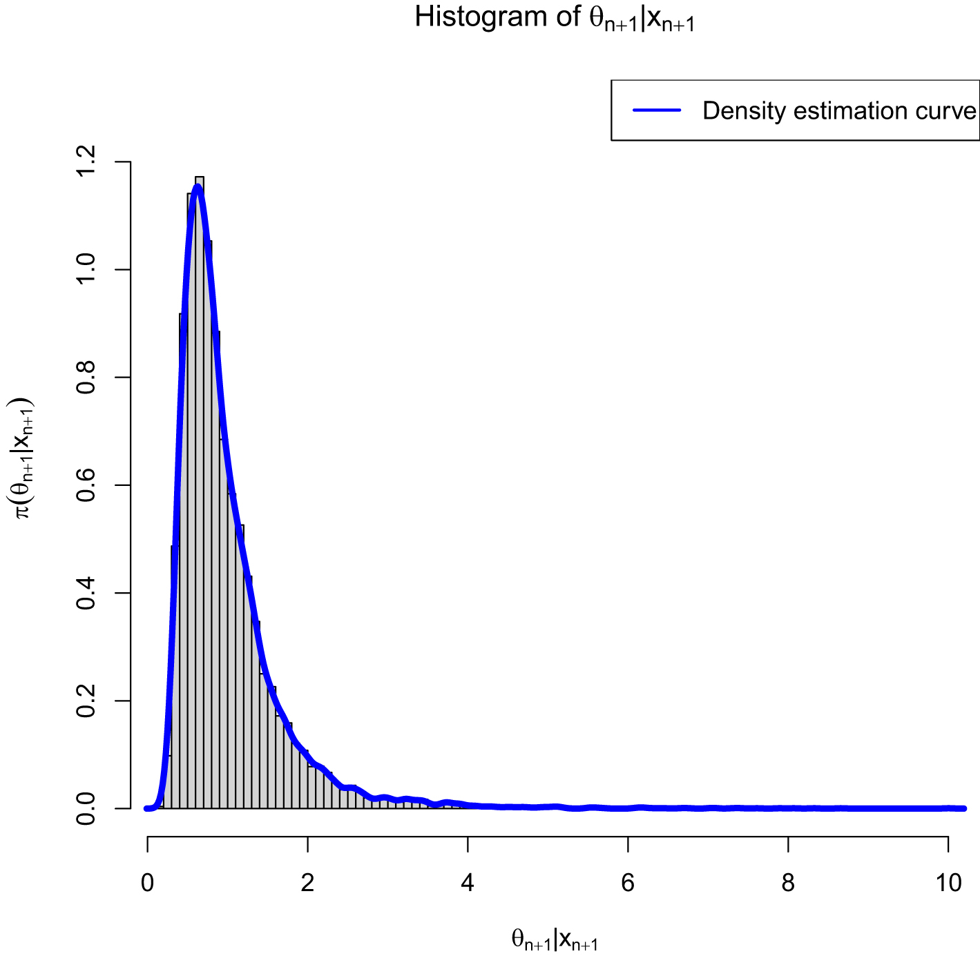
, , and . Figure 4.1 shows the histogram of and the density estimation curve of . It is that we find to minimize the PESL. Numerical results show that
FIG. 4.1 — Exp-IG: The histogram of  and the density estimation curve of
  .
.
and the density estimation curve of .
Second, let us allow one of the quantities  ,
,  , and
, and  to change, holding other quantities fixed. Figure 4.2 shows the Bayes estimators and the PESLs as functions of
  ,
,  , and
, and  . We see from the left plots of the figure that the Bayes estimators depend on
  ,
,  , and
, and  , and (4.8) is exemplified. More specifically, the Bayes estimators are decreasing functions of
  , linearly increasing functions of
  , and linearly increasing functions of
  . The right plots of the figure exhibit that the PESLs depend only on
  , but not on
  and
and  , and (4.11) is exemplified. More specifically, the PESLs are decreasing functions of
  . Furthermore, tables 4.1–4.3 display the numerical values of the Bayes estimators and the PESLs in figure 4.2. In summary, the results of figure 4.2 and tables 4.1–4.3 exemplify the theoretical studies of (4.8) and (4.11).
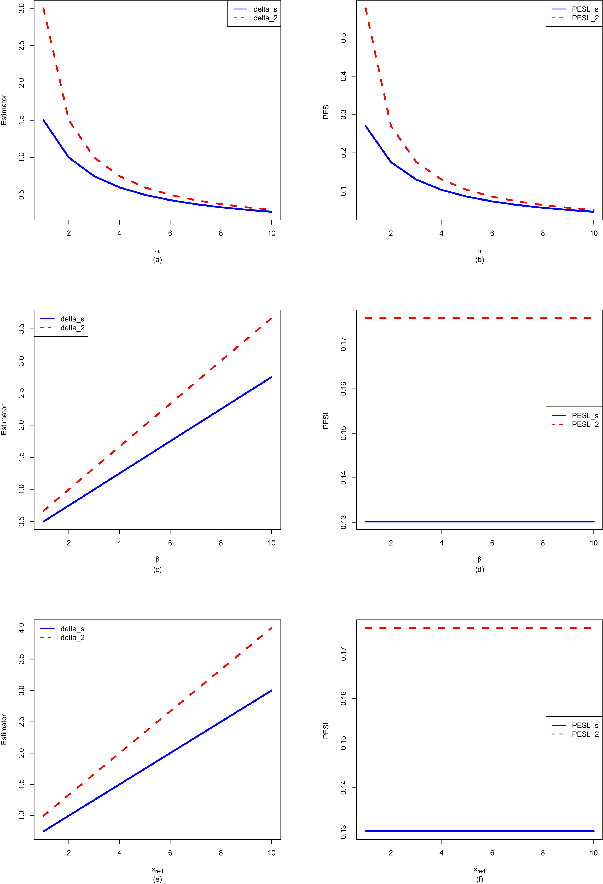
, , and to change, holding other quantities fixed. Figure 4.2 shows the Bayes estimators and the PESLs as functions of , , and . We see from the left plots of the figure that the Bayes estimators depend on , , and , and (4.8) is exemplified. More specifically, the Bayes estimators are decreasing functions of , linearly increasing functions of , and linearly increasing functions of . The right plots of the figure exhibit that the PESLs depend only on , but not on and , and (4.11) is exemplified. More specifically, the PESLs are decreasing functions of . Furthermore, tables 4.1–4.3 display the numerical values of the Bayes estimators and the PESLs in figure 4.2. In summary, the results of figure 4.2 and tables 4.1–4.3 exemplify the theoretical studies of (4.8) and (4.11).
FIG. 4.2 — Exp-IG: The Bayes estimators and the PESLs as functions of  ,
,  , and
, and  . (a) Bayes estimators vs.
  . (b) PESLs vs.
 . (c) Bayes estimators vs.
  . (d) PESLs vs.
  . (e) Bayes estimators vs.
  . (f) PESLs vs.
  .
.
, , and . (a) Bayes estimators vs. . (b) PESLs vs.. (c) Bayes estimators vs. . (d) PESLs vs. . (e) Bayes estimators vs. . (f) PESLs vs. .
TAB. 4.1 — Exp-IG: The numerical values of the Bayes estimators and the PESLs in figure 4.2:  changes.
changes.
 |
1 | 2 | 3 | 4 | 5 | 6 | 7 | 8 | 9 | 10 |
 |
1.5000 | 1.0000 | 0.7500 | 0.6000 | 0.5000 | 0.4286 | 0.3750 | 0.3333 | 0.3000 | 0.2727 |
 |
3.0000 | 1.5000 | 1.0000 | 0.7500 | 0.6000 | 0.5000 | 0.4286 | 0.3750 | 0.3333 | 0.3000 |
 |
0.2704 | 0.1758 | 0.1302 | 0.1033 | 0.0856 | 0.0731 | 0.0638 | 0.0566 | 0.0508 | 0.0461 |
 |
0.5772 | 0.2704 | 0.1758 | 0.1302 | 0.1033 | 0.0856 | 0.0731 | 0.0638 | 0.0566 | 0.0508 |
TAB. 4.2 — Exp-IG: The numerical values of the Bayes estimators and the PESLs in figure 4.2:  changes.
changes.
 |
1 | 2 | 3 | 4 | 5 | 6 | 7 | 8 | 9 | 10 |
 |
0.5000 | 0.7500 | 1.0000 | 1.2500 | 1.5000 | 1.7500 | 2.0000 | 2.2500 | 2.5000 | 2.7500 |
 |
0.6667 | 1.0000 | 1.3333 | 1.6667 | 2.0000 | 2.3333 | 2.6667 | 3.0000 | 3.3333 | 3.6667 |
 |
0.1302 | 0.1302 | 0.1302 | 0.1302 | 0.1302 | 0.1302 | 0.1302 | 0.1302 | 0.1302 | 0.1302 |
 |
0.1758 | 0.1758 | 0.1758 | 0.1758 | 0.1758 | 0.1758 | 0.1758 | 0.1758 | 0.1758 | 0.1758 |
TAB. 4.3 — Exp-IG: The numerical values of the Bayes estimators and the PESLs in figure 4.2:  changes.
changes.
 |
1 | 2 | 3 | 4 | 5 | 6 | 7 | 8 | 9 | 10 |
 |
0.7500 | 1.0000 | 1.2500 | 1.5000 | 1.7500 | 2.0000 | 2.2500 | 2.5000 | 2.7500 | 3.0000 |
 |
1.0000 | 1.3333 | 1.6667 | 2.0000 | 2.3333 | 2.6667 | 3.0000 | 3.3333 | 3.6667 | 4.0000 |
 |
0.1302 | 0.1302 | 0.1302 | 0.1302 | 0.1302 | 0.1302 | 0.1302 | 0.1302 | 0.1302 | 0.1302 |
 |
0.1758 | 0.1758 | 0.1758 | 0.1758 | 0.1758 | 0.1758 | 0.1758 | 0.1758 | 0.1758 | 0.1758 |
Third, since the Bayes estimators  and
and  and the PESLs
  and
and  depend on
  and
and  , where
  and
and  , we can plot the surfaces of the Bayes estimators and the PESLs on the domain
  via the R function persp3d() in the R package rgl (see Zhang et al. (2017, 2019b); Adler et al. (2017)). We remark that the R function persp() in the R package graphics can not add another surface to the existing surface, but persp3d() can. Moreover, persp3d() allows one to rotate the perspective plots of the surface according to one’s wishes. Figure 4.3 plots the surfaces of the Bayes estimators and the PESLs, and the surfaces of the differences of the Bayes estimators and the PESLs. The domain for
  is
is  for all the plots. a is for
  and b is for
  in the axes of all the plots. The red surface is for
  and the blue surface is for
  in the upper two plots. From the left two plots of the figure, we see that
  for all
  on
on  . From the right two plots of the figure, we see that
  for all
  on
on  . The results of figure 4.3 exemplify the theoretical studies of (4.8) and (4.11).
and and the PESLs and depend on and , where and , we can plot the surfaces of the Bayes estimators and the PESLs on the domain via the R function persp3d() in the R package rgl (see Zhang et al. (2017, 2019b); Adler et al. (2017)). We remark that the R function persp() in the R package graphics can not add another surface to the existing surface, but persp3d() can. Moreover, persp3d() allows one to rotate the perspective plots of the surface according to one’s wishes. Figure 4.3 plots the surfaces of the Bayes estimators and the PESLs, and the surfaces of the differences of the Bayes estimators and the PESLs. The domain for is for all the plots. a is for and b is for in the axes of all the plots. The red surface is for and the blue surface is for in the upper two plots. From the left two plots of the figure, we see that for all on . From the right two plots of the figure, we see that for all on . The results of figure 4.3 exemplify the theoretical studies of (4.8) and (4.11).
4.3.2 Consistencies of the Moment Estimators and the MLEs
In this subsection, similar to subsection 1.8.1, we will numerically exemplify that the moment estimators and the MLEs are consistent estimators of the hyperparameters  and
and  of the hierarchical exponential and inverse gamma (4.1). The motivation of this subsection is that in Theorems 4.2 and 4.3, we have theoretically shown that the moment estimators and the MLEs are consistent estimators of the hyperparameters. Note that only
  are used in this subsection.
and of the hierarchical exponential and inverse gamma (4.1). The motivation of this subsection is that in Theorems 4.2 and 4.3, we have theoretically shown that the moment estimators and the MLEs are consistent estimators of the hyperparameters. Note that only are used in this subsection.
The frequencies of the moment estimators ( and
and  ) and the MLEs (
 and
and  ) of the hyperparameters (
 and
and  ) as
) as  varies for
  and
and  , 0.5, and 0.1 are reported in table 4.4. From the table, we observe the following facts.
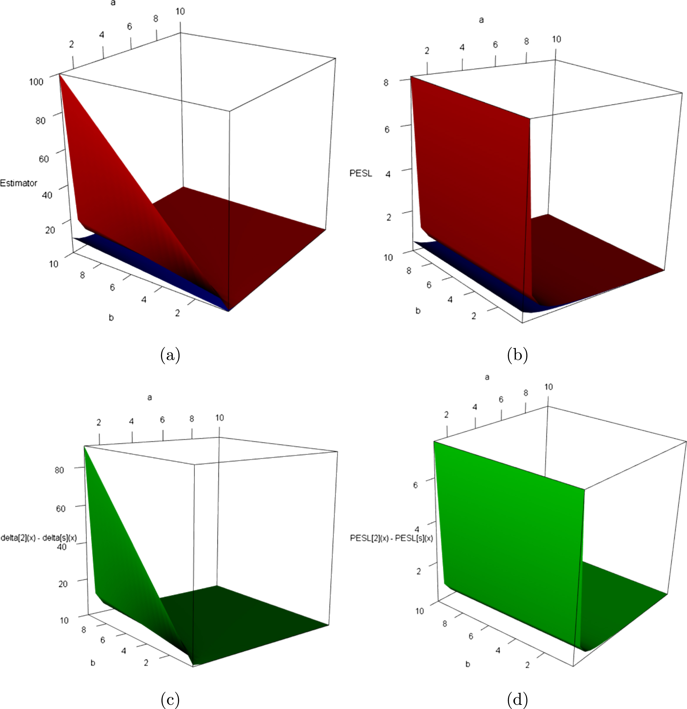
and ) and the MLEs ( and ) of the hyperparameters ( and ) as varies for and , 0.5, and 0.1 are reported in table 4.4. From the table, we observe the following facts.
FIG. 4.3 — Exp-IG: (a) The Bayes estimators as functions of  and
and  . (b) The PESLs as functions of
  and
and  . (c) The surface of
  which is positive for all
  on
on  . (d) The surface of
  which is also positive for all
  on
on  .
.
and . (b) The PESLs as functions of and . (c) The surface of which is positive for all on . (d) The surface of which is also positive for all on .
1. Given  , 0.5, or 0.1, the frequencies (
 ,
,  or
or  ,
,  ) of the estimators tend to 0 as
  increases to infinity, which means that the moment estimators and the MLEs are consistent estimators of the hyperparameters. For
  , the frequencies of the estimators are still very large. However, we observe the tendency to decline to 0 as
  increases to infinity.
, 0.5, or 0.1, the frequencies (, or , ) of the estimators tend to 0 as increases to infinity, which means that the moment estimators and the MLEs are consistent estimators of the hyperparameters. For , the frequencies of the estimators are still very large. However, we observe the tendency to decline to 0 as increases to infinity.
2. Comparing the frequencies corresponding to  , 0.5, and 0.1, we observe that as
  gets smaller, the frequencies tend to be larger, since the constraints
 are easier to meet.
, 0.5, and 0.1, we observe that as gets smaller, the frequencies tend to be larger, since the constraints
3. Comparing the moment estimators and the MLEs of the hyperparameters  and
and  , we see that the frequencies of the MLEs are smaller than those of the moment estimators, which means that the MLEs are better than the moment estimators when estimating the hyperparameters in terms of consistency.
and , we see that the frequencies of the MLEs are smaller than those of the moment estimators, which means that the MLEs are better than the moment estimators when estimating the hyperparameters in terms of consistency.
4.3.3 Goodness-of-Fit of the Model: KS Test
In this subsection, similar to subsection 1.8.2, we will calculate the goodness-of-fit of the hierarchical exponential and inverse gamma model (4.1) to the simulated data. The motivation of this subsection is that we want to check whether the marginal distribution of the hierarchical exponential and inverse gamma model (4.1) fits the simulated data well. Note that only  are used in this subsection.
are used in this subsection.
In our problem, the null hypothesis specifies that
 where
where  is the marginal distribution of the hierarchical exponential and inverse gamma model (4.1). The marginal density of the
  distribution is given by (4.5) which is obviously one-dimensional continuous. Hence, the KS test can be utilized as a measure of the goodness-of-fit.
is the marginal distribution of the hierarchical exponential and inverse gamma model (4.1). The marginal density of the distribution is given by (4.5) which is obviously one-dimensional continuous. Hence, the KS test can be utilized as a measure of the goodness-of-fit.
TAB. 4.4 — Exp-IG: The frequencies of the moment estimators and the MLEs of the hyperparameters as  varies for
  and
and  , 0.5, and 0.1.
varies for and , 0.5, and 0.1.
| Moment estimators | MLEs | ||||
 |
 |
 |
 |
 |
|
 |
1e4 | 0.00 | 0.00 | 0.00 | 0.00 |
| 2e4 | 0.00 | 0.00 | 0.00 | 0.00 | |
| 4e4 | 0.00 | 0.00 | 0.00 | 0.00 | |
| 8e4 | 0.00 | 0.00 | 0.00 | 0.00 | |
 |
1e4 | 0.14 | 0.11 | 0.00 | 0.00 |
| 2e4 | 0.02 | 0.01 | 0.00 | 0.00 | |
| 4e4 | 0.01 | 0.01 | 0.00 | 0.00 | |
| 8e4 | 0.00 | 0.00 | 0.00 | 0.00 | |
 |
1e4 | 0.77 | 0.74 | 0.40 | 0.31 |
| 2e4 | 0.70 | 0.69 | 0.24 | 0.15 | |
| 4e4 | 0.64 | 0.62 | 0.13 | 0.09 | |
| 8e4 | 0.48 | 0.46 | 0.03 | 0.01 | |
The results of the KS test goodness-of-fit of the model (4.1) to the simulated data are reported in table 4.5. Note that the data are simulated according to the hierarchical exponential and inverse gamma model (4.1) with  and
and  . In the table, the hyperparameters
  and
and  are estimated by three methods. The first method is the oracle method, in that we know the hyperparameters
  and
and  . The second method is the moment method, in that the hyperparameters
  and
and  are estimated by their moment estimators (see Theorem 4.2). The third method is the MLE method, in which the hyperparameters
  and
and  are estimated by their MLEs (see Theorem 4.3). In the table, the sample size is
  , and the number of simulations is
  .
.
and . In the table, the hyperparameters and are estimated by three methods. The first method is the oracle method, in that we know the hyperparameters and . The second method is the moment method, in that the hyperparameters and are estimated by their moment estimators (see Theorem 4.2). The third method is the MLE method, in which the hyperparameters and are estimated by their MLEs (see Theorem 4.3). In the table, the sample size is , and the number of simulations is .
From table 4.5, we observe the following facts.
1. The  values for the three methods are respectively given by 0.0270, 0.0230, and 0.0205, which means that the MLE method is the best method, the moment method is the second-best method, and the oracle method is the worst method. A possible explanation for this phenomenon is that in (1.23), the empirical cdf
  is based on data, and the population cdfs
  for the MLE method and the moment method are also based on data, while the population cdf
  for the oracle method is not based on data.
values for the three methods are respectively given by 0.0270, 0.0230, and 0.0205, which means that the MLE method is the best method, the moment method is the second-best method, and the oracle method is the worst method. A possible explanation for this phenomenon is that in (1.23), the empirical cdf is based on data, and the population cdfs for the MLE method and the moment method are also based on data, while the population cdf for the oracle method is not based on data.
2. The  values for the three methods are respectively given by 0.5102, 0.6683, and 0.7693, which also means that the MLE method ranks first, the moment method ranks second, and the oracle method ranks third. The possible explanation for this phenomenon is described in the previous paragraph.
values for the three methods are respectively given by 0.5102, 0.6683, and 0.7693, which also means that the MLE method ranks first, the moment method ranks second, and the oracle method ranks third. The possible explanation for this phenomenon is described in the previous paragraph.
3. The  values for the three methods are respectively given by 0.16, 0.15, and 0.69. The
  value for the MLE method accounts for over half of the
  simulations. The order of preference for the three methods is the MLE method, the oracle method, and the moment method.
values for the three methods are respectively given by 0.16, 0.15, and 0.69. The value for the MLE method accounts for over half of the simulations. The order of preference for the three methods is the MLE method, the oracle method, and the moment method.
4. The  values for the three methods are respectively given by 0.16, 0.15, and 0.69. A small
  value corresponds to a large p-value. Hence, the smallest
  value corresponds to the largest p-value. Therefore, the
  value and the
  value for the three methods are the same. The order of preference for the three methods is the MLE method, the oracle method, and the moment method.
values for the three methods are respectively given by 0.16, 0.15, and 0.69. A small value corresponds to a large p-value. Hence, the smallest value corresponds to the largest p-value. Therefore, the value and the value for the three methods are the same. The order of preference for the three methods is the MLE method, the oracle method, and the moment method.
5. The  values for the three methods are respectively given by 0.97, 0.99, and 1.00. Once again, the order of preference for the three methods is the MLE method, the moment method, and the oracle method.
values for the three methods are respectively given by 0.97, 0.99, and 1.00. Once again, the order of preference for the three methods is the MLE method, the moment method, and the oracle method.
TAB. 4.5 — Exp-IG: The results of the KS test goodness-of-fit of the model (4.1) to the simulated data.
 |
 |
 |
|
 |
0.0270 | 0.0230 | 0.0205 |
 |
0.5102 | 0.6683 | 0.7693 |
 |
0.16 | 0.15 | 0.69 |
 |
0.16 | 0.15 | 0.69 |
 |
0.97 | 0.99 | 1.00 |
The boxplots of the  values and the p-values for the three methods are displayed in figure 4.4. From the figure, we observe the following facts.
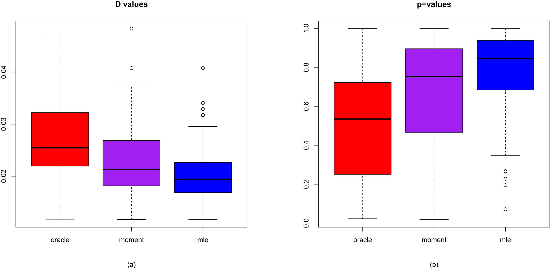
values and the p-values for the three methods are displayed in figure 4.4. From the figure, we observe the following facts.
1. The  values of the oracle method are significantly larger than those of the other two methods. Since for the
  value, the smaller the better, the order of preference for the three methods is the MLE method, the moment method, and the oracle method.
values of the oracle method are significantly larger than those of the other two methods. Since for the value, the smaller the better, the order of preference for the three methods is the MLE method, the moment method, and the oracle method.
2. The p-values of the oracle method are significantly smaller than those of the other two methods. Since for the p-value, the larger the better, the order of preference for the three methods is the MLE method, the moment method, and the oracle method.
3. Small  values correspond to large p-values, and large
  values correspond to small p-values.
values correspond to large p-values, and large values correspond to small p-values.
4. The MLE method has a better performance than the moment method in terms of the  values and the p-values.
values and the p-values.
FIG. 4.4 — Exp-IG: The boxplots of the  values and the p-values for the three methods. (a)
  values. (b) p-values.
values and the p-values for the three methods. (a) values. (b) p-values.
4.3.4 Numerical Comparisons of the Bayes Estimators and the PESLs of Three Methods
In this subsection, we will numerically compare the Bayes estimators and the PESLs of three methods (the oracle method, the moment method, and the MLE method). The motivation of this subsection is that the theoretical comparisons of the Bayes estimators and the PESLs of the three methods can be found in subsection 4.2.3.
Note that the data are simulated according to the hierarchical exponential and inverse gamma model (4.1) with  and
and  . Moreover, the oracle method knows the hyperparameters
  and
and  in simulations.
and . Moreover, the oracle method knows the hyperparameters and in simulations.
Comparisons of  ,
,  ,
,  ,
,  ,
,  , and
, and  of the three methods for sample size
  and the number of simulations
  are displayed in figure 4.5. From the figure, we observe the following facts.
, , , , , and of the three methods for sample size and the number of simulations are displayed in figure 4.5. From the figure, we observe the following facts.
1. For the estimators of  and
and  , the MLE method is much closer to the oracle method than the moment method.
and , the MLE method is much closer to the oracle method than the moment method.
2. For the Bayes estimators  and
and 
 , the MLE method is slightly closer to the oracle method than the moment method. The three curves are almost indistinguishable, as the differences among the estimators are negligible.
and , the MLE method is slightly closer to the oracle method than the moment method. The three curves are almost indistinguishable, as the differences among the estimators are negligible.
3. For the PESLs  and
and 
 , the MLE method is much closer to the oracle method than the moment method.
and , the MLE method is much closer to the oracle method than the moment method.
4. All the plots indicate that the MLE method is better than the moment method, as the estimators of the hyperparameters, the Bayes estimators, and the PESLs of the MLE method are closer to those of the oracle method than those of the moment method.
The boxplots of the absolute errors from the oracle method by the moment method and the MLE method for sample size  and number of simulations
  are displayed in figure 4.6. All the plots indicate that the MLE method is better than the moment method, as the absolute errors from the oracle method of the estimators of the hyperparameters, the Bayes estimators, and the PESLs by the MLE method are much smaller than those by the moment method.
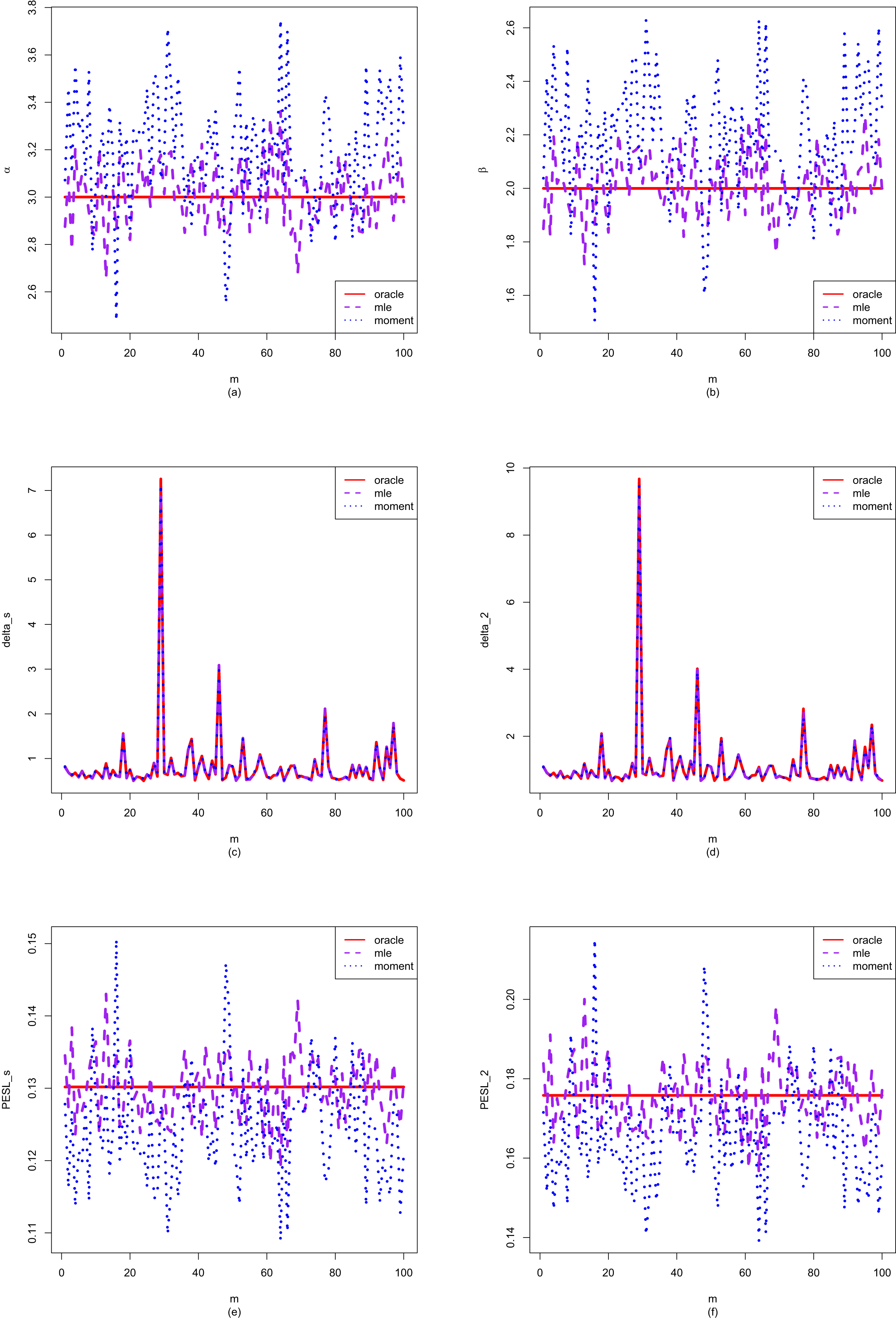
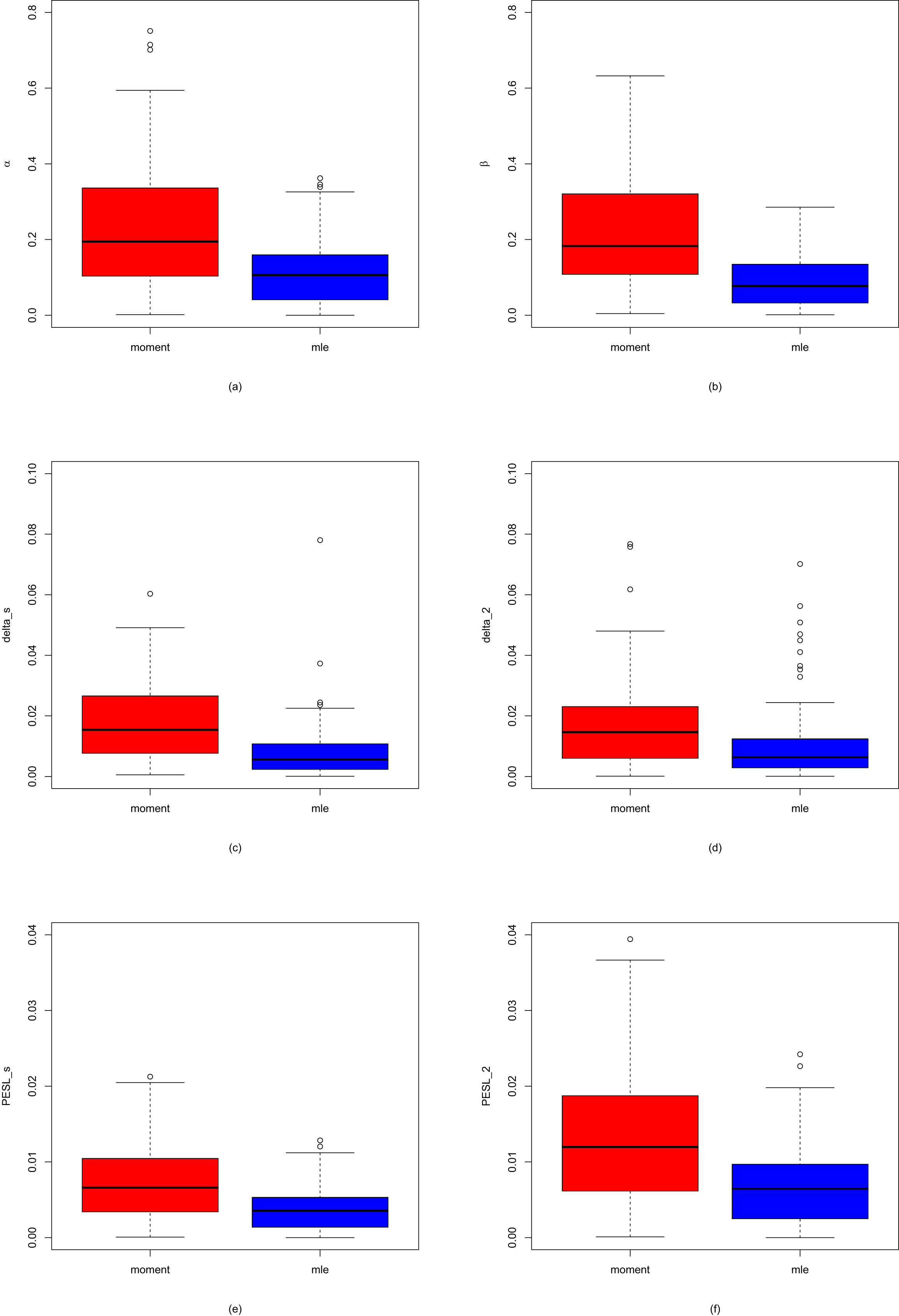
and number of simulations are displayed in figure 4.6. All the plots indicate that the MLE method is better than the moment method, as the absolute errors from the oracle method of the estimators of the hyperparameters, the Bayes estimators, and the PESLs by the MLE method are much smaller than those by the moment method.
FIG. 4.5 — Exp-IG: Comparisons of  ,
,  ,
,  ,
,  ,
,  , and
, and  of the three methods for sample size
  and number of simulations
  . (a)
. (a)  . (b)
. (b)  . (c)
. (c)  . (d)
. (d)  . (e)
. (e)  . (f)
. (f)  .
.
, , , , , and of the three methods for sample size and number of simulations . (a) . (b) . (c) . (d) . (e) . (f) .
FIG. 4.6 — Exp-IG: The boxplots of the absolute errors from the oracle method by the moment method and the MLE method for sample size  and number of simulations
  . (a)
. (a)  . (b)
. (b)  . (c)
. (c)  . (d)
. (d)  . (e)
. (e)  . (f)
. (f)  .
.
and number of simulations . (a) . (b) . (c) . (d) . (e) . (f) .
The averages and proportions of the absolute errors from the oracle method by the moment method and the MLE method for the estimators of the hyperparameters, the Bayes estimators, and the PESLs are summarized in table 4.6. See subsection 1.8.3 for details. From the table, we observe that the averages of the absolute errors from the oracle method by the MLE method are much smaller than those by the moment method. Moreover, the proportions of the absolute errors from the oracle method by the MLE method are much larger than those by the moment method. In summary, the table illustrates that the MLE method is better than the moment method in terms of the averages and proportions of the absolute errors from the oracle method.
TAB. 4.6 — Exp-IG: The averages and proportions of the absolute errors from the oracle method by the moment method and the MLE method for the estimators of the hyperparameters, the Bayes estimators, and the PESLs.
| Averages | Proportions | |||
| Moment | MLE | Moment | MLE | |
 |
0.2458 | 0.1099 | 0.28 | 0.72 |
 |
0.2354 | 0.0931 | 0.21 | 0.79 |
 |
0.0199 | 0.0106 | 0.22 | 0.78 |
 |
0.0210 | 0.0167 | 0.37 | 0.63 |
 |
0.0077 | 0.0037 | 0.28 | 0.72 |
 |
0.0138 | 0.0067 | 0.28 | 0.72 |
The MSE and MAE of the estimators of the hyperparameters by the moment method and the MLE method are summarized in table 4.7. See subsection 1.8.3 for details. From the table, we see that the MLE method is far better than the moment method when estimating the hyperparameters  and
and  , as the MSE and MAE by the MLE method are much smaller than those by the moment method.
and , as the MSE and MAE by the MLE method are much smaller than those by the moment method.
TAB. 4.7 — Exp-IG: The MSE and MAE of the estimators of the hyperparameters by the moment method and the MLE method.
| MSE | MAE | |||
| Moment | MLE | Moment | MLE | |
 |
0.09178 | 0.01877 | 0.24582 | 0.10993 |
 |
0.08204 | 0.01363 | 0.23538 | 0.09313 |
4.3.5 Marginal Densities for Various Hyperparameters
In this subsection, we will plot the marginal densities of the hierarchical exponential and inverse gamma model (4.1) for various hyperparameters  and
and  . The motivation of this subsection is that we want to know what kind of data can be modeled by the hierarchical exponential and inverse gamma model (4.1). Note that the marginal density of
  is given by (4.5) specified by two hyperparameters
  and
and  . We will explore how the marginal densities change around the marginal density with the hyperparameters specified by
  and
and  . Other numerical values of the hyperparameters can also be specified.
and . The motivation of this subsection is that we want to know what kind of data can be modeled by the hierarchical exponential and inverse gamma model (4.1). Note that the marginal density of is given by (4.5) specified by two hyperparameters and . We will explore how the marginal densities change around the marginal density with the hyperparameters specified by and . Other numerical values of the hyperparameters can also be specified.
Figure 4.7 plots the marginal densities for varied  , holding
  fixed. From the figure, we see that as
  increases, the peak value of the curve increases. In other words, the variance of the marginal density decreases, as
 (4.16)
is a decreasing function of
(4.16)
is a decreasing function of  . Moreover, all the marginal densities are decreasing functions of
  and right skewed.
, holding fixed. From the figure, we see that as increases, the peak value of the curve increases. In other words, the variance of the marginal density decreases, as
(4.16)
. Moreover, all the marginal densities are decreasing functions of and right skewed.
Figure 4.8 plots the marginal densities for varied  , holding
  fixed. From the figure, we see that as
  increases, the peak value of the curve decreases. In other words, the variance of the marginal density increases, as (4.16) is an increasing function of
  . Moreover, all the marginal densities are also decreasing functions of
  and right skewed.
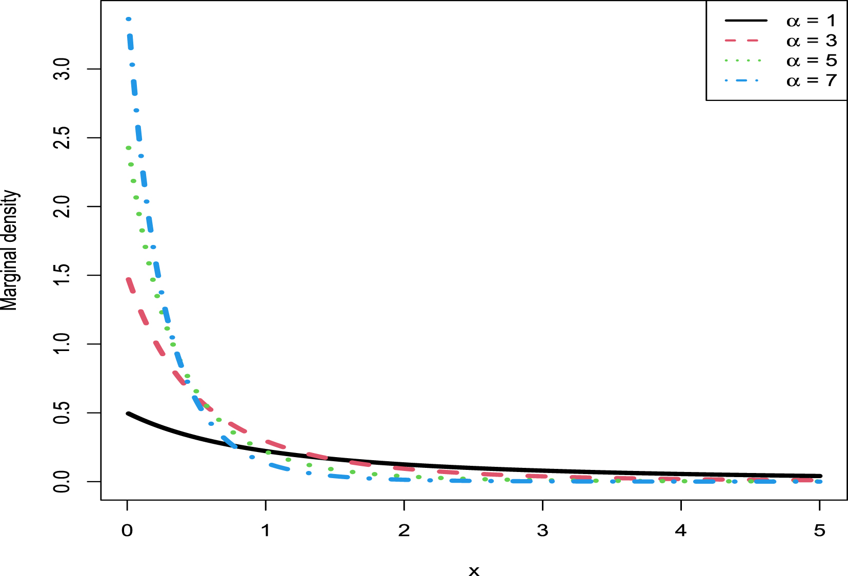
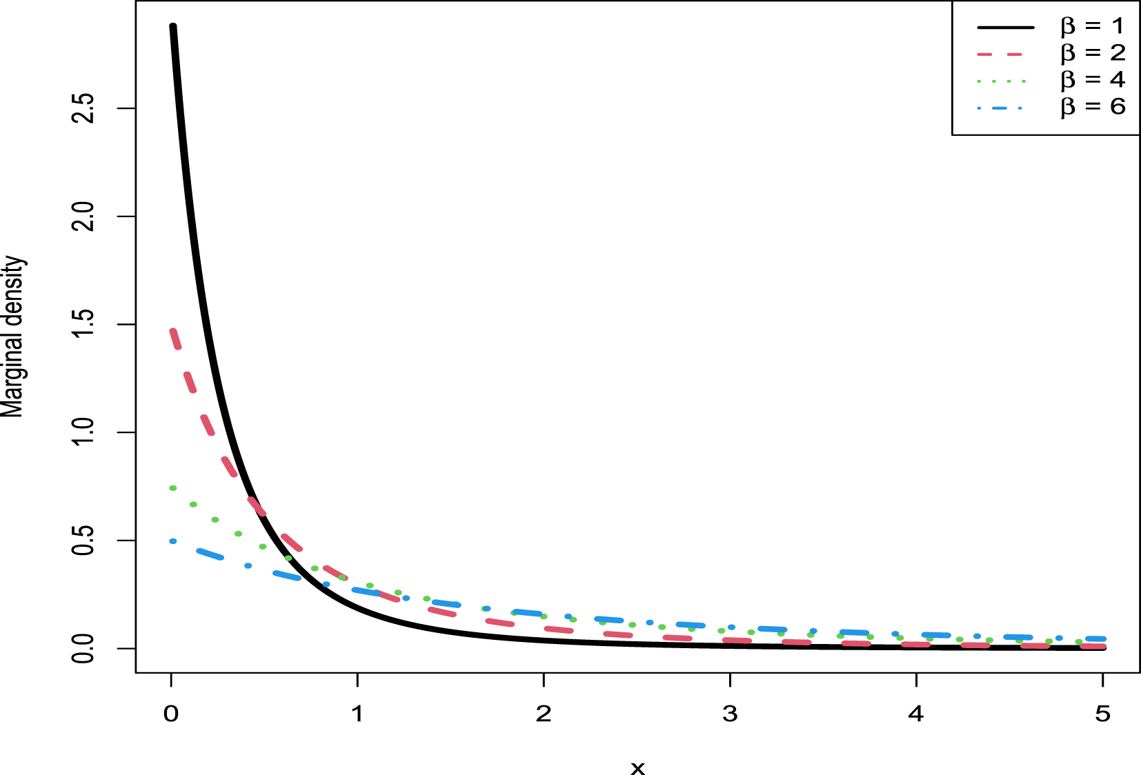
, holding fixed. From the figure, we see that as increases, the peak value of the curve decreases. In other words, the variance of the marginal density increases, as (4.16) is an increasing function of . Moreover, all the marginal densities are also decreasing functions of and right skewed.
FIG. 4.7 — Exp-IG: The marginal densities for varied  , holding
  fixed.
, holding fixed.
FIG. 4.8 — Exp-IG: The marginal densities for varied  , holding
  fixed.
, holding fixed.
4.4 A Real Data Example
In this section, we utilize the Static Fatigue  Stress Level data to illustrate our methods (see R. E. Barlow University of California, Berkeley (2021)). Kevlar Epoxy is a material used on the National Aeronautics and Space Administration (NASA) space shuttle. Strands of this epoxy were tested at 90% breaking strength. The data represent time to failure in hours at the 90% stress level for a random sample of 50
  epoxy strands. The data used to support the findings of this study are available at https://college.cengage.com/mathematics/brase/understandable_statistics/7e/students/datasets/svls/frames/frame.html.
Stress Level data to illustrate our methods (see R. E. Barlow University of California, Berkeley (2021)). Kevlar Epoxy is a material used on the National Aeronautics and Space Administration (NASA) space shuttle. Strands of this epoxy were tested at 90% breaking strength. The data represent time to failure in hours at the 90% stress level for a random sample of 50 epoxy strands. The data used to support the findings of this study are available at https://college.cengage.com/mathematics/brase/understandable_statistics/7e/students/datasets/svls/frames/frame.html.
The histogram of the sample  (the Static Fatigue
  Stress Level data) along with its density estimation curve are depicted in Figure 4.9. From the figure we see that the histogram is roughly decreasing, and thus the hierarchical exponential and inverse gamma model (4.1) should be appropriate. See subsection “Marginal densities for various hyperparameters" for details.
(the Static Fatigue Stress Level data) along with its density estimation curve are depicted in Figure 4.9. From the figure we see that the histogram is roughly decreasing, and thus the hierarchical exponential and inverse gamma model (4.1) should be appropriate. See subsection “Marginal densities for various hyperparameters" for details.
The estimators of the hyperparameters  and
and  , the goodness-of-fit of the model, the empirical Bayes estimators of the mean parameter of the exponential distribution with a conjugate inverse gamma prior and the PESLs, and the mean and variance of the Static Fatigue
  Stress Level data by the moment method and the MLE method are summarized in table 4.8. From the table, we observe the following facts.
and , the goodness-of-fit of the model, the empirical Bayes estimators of the mean parameter of the exponential distribution with a conjugate inverse gamma prior and the PESLs, and the mean and variance of the Static Fatigue Stress Level data by the moment method and the MLE method are summarized in table 4.8. From the table, we observe the following facts.
1. The moment estimators and the MLEs of the hyperparameters  and
and  are quite different. This does not mean that the hierarchical exponential and inverse gamma model (4.1) does not fit the real data, nor mean that the moment estimators and the MLEs are not consistent estimators of the hyperparameters
  and
and  . The reason for the big differences between the two estimators is that the sample size
  is too small. Of course, the MLEs of the hyperparameters
  and
and  are more reliable, as assured from the previous figures and tables in the simulations section.
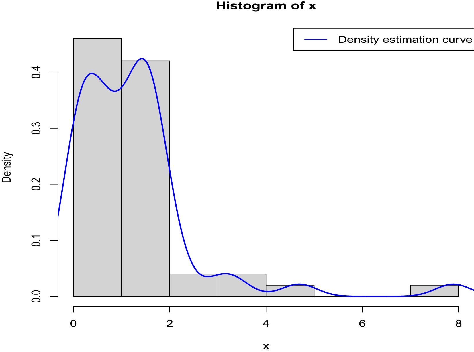
and are quite different. This does not mean that the hierarchical exponential and inverse gamma model (4.1) does not fit the real data, nor mean that the moment estimators and the MLEs are not consistent estimators of the hyperparameters and . The reason for the big differences between the two estimators is that the sample size is too small. Of course, the MLEs of the hyperparameters and are more reliable, as assured from the previous figures and tables in the simulations section.
FIG. 4.9 — Exp-IG: The histogram of the sample  along with its density estimation curve.
along with its density estimation curve.
2. We use the KS test as a measure of the goodness-of-fit. The p-value of the moment method is  , and thus the
  distribution with
  and
and  estimated by their moment estimators fits the sample
  well. Moreover, the p-value of the MLE method is
  , and thus the
  distribution with
  and
and  estimated by their MLEs fits the sample
  well. When comparing the two methods, we observe that the
  value of the MLEs is smaller, and the p-value of the MLEs is larger, which means that the
  distribution with
  and
and  estimated by the MLEs has a better fit to the sample
  than that estimated by the moment estimators.
, and thus the distribution with and estimated by their moment estimators fits the sample well. Moreover, the p-value of the MLE method is , and thus the distribution with and estimated by their MLEs fits the sample well. When comparing the two methods, we observe that the value of the MLEs is smaller, and the p-value of the MLEs is larger, which means that the distribution with and estimated by the MLEs has a better fit to the sample than that estimated by the moment estimators.
3. When the hyperparameters are estimated by the MLE method, we see that
 and
and

When the hyperparameters are estimated by the moment method, we observe a similar phenomenon for the Bayes estimators and the PESLs. Consequently, the two inequalities (4.8) and (4.11) are exemplified.
4. The mean of  (the Static Fatigue 90% Stress Level data) is estimated by
 for
for  . The variance of
  is estimated by
 for
for  . It is interesting to note that the mean and variance of
  by the two methods are very similar, although the estimators of the hyperparameters are quite different. Moreover, it is easy to see that
 for the MLE method. The mean and variance of
  are similar for the moment method.
(the Static Fatigue 90% Stress Level data) is estimated by
. The variance of is estimated by
. It is interesting to note that the mean and variance of by the two methods are very similar, although the estimators of the hyperparameters are quite different. Moreover, it is easy to see that
are similar for the moment method.
TAB. 4.8 — Exp-IG: The estimators of the hyperparameters, the goodness-of-fit of the model, the empirical Bayes estimators of the mean parameter of the exponential distribution with a conjugate inverse gamma prior and the PESLs, and the mean and variance of the Static Fatigue 90% Stress Level data by the moment method and the MLE method.
| Moment method | MLE method | ||
| Estimators of |  |
 |
 |
| the hyperparameters |  |
 |
 |
| Goodness-of-fit |  |
0.1240 | 0.1209 |
| of the model | p-value | 0.4389 | 0.4708 |
| Empirical Bayes estimators |  |
1.156655 | 1.179281 |
| and PESLs |  |
1.222516 | 1.229669 |
 |
0.027179 | 0.020628 | |
 |
0.028741 | 0.021516 | |
| Mean and variance of |  |
1.252857 | 1.252418 |
| the Static Fatigue 90% Stress Level data |  |
1.771380 | 1.715116 |
4.5 Conclusions and Discussions
For the hierarchical exponential and inverse gamma model (4.1), we calculate the posterior density  and the marginal density
  in Theorem 4.1. After that, we calculate the Bayes estimators of
  ,
,  and
and  , and the PESLs of
  ,
,  and
and  . Moreover, they satisfy two inequalities (4.8) and (4.11). The estimators of the hyperparameters of the model (4.1) by the moment method and their consistencies are summarized in Theorem 4.2. Furthermore, the estimators of the hyperparameters of the model (4.1) by the MLE method and their consistencies are summarized in Theorem 4.3. Finally, the empirical Bayes estimators of the parameter of the model (4.1) under Stein’s loss function by the moment method and the MLE method are summarized in Theorem 4.4.
and the marginal density in Theorem 4.1. After that, we calculate the Bayes estimators of , and , and the PESLs of , and . Moreover, they satisfy two inequalities (4.8) and (4.11). The estimators of the hyperparameters of the model (4.1) by the moment method and their consistencies are summarized in Theorem 4.2. Furthermore, the estimators of the hyperparameters of the model (4.1) by the MLE method and their consistencies are summarized in Theorem 4.3. Finally, the empirical Bayes estimators of the parameter of the model (4.1) under Stein’s loss function by the moment method and the MLE method are summarized in Theorem 4.4.
In the simulations section, we have illustrated five aspects. First, we have numerically exemplified two inequalities (4.8) and (4.11) of the Bayes estimators and the PESLs. Second, we have illustrated that the moment estimators and the MLEs are consistent estimators of the hyperparameters. Third, we have calculated the goodness-of-fit of the model to the simulated data by the KS test. Fourth, we have numerically compared the Bayes estimators and the PESLs of the three methods (the oracle method, the moment method, and the MLE method). Finally, we have plotted the marginal densities of the model for various hyperparameters.
We utilize the Static Fatigue 90% Stress Level data to illustrate our methods. The estimators of the hyperparameters  and
and  , the goodness-of-fit of the model, the empirical Bayes estimators of the mean parameter of the exponential distribution with a conjugate inverse gamma prior and the PESLs, and the mean and variance of the Static Fatigue
  Stress Level data by the moment method and the MLE method are summarized in table 4.8. The
  distribution with the hyperparameters
  and
and  estimated by the MLEs has a better goodness-of-fit to the sample
  than that estimated by the moment estimators. Moreover, the two inequalities (4.8) and (4.11) are exemplified for the sample
  .
.
and , the goodness-of-fit of the model, the empirical Bayes estimators of the mean parameter of the exponential distribution with a conjugate inverse gamma prior and the PESLs, and the mean and variance of the Static Fatigue Stress Level data by the moment method and the MLE method are summarized in table 4.8. The distribution with the hyperparameters and estimated by the MLEs has a better goodness-of-fit to the sample than that estimated by the moment estimators. Moreover, the two inequalities (4.8) and (4.11) are exemplified for the sample .
Chapter 5 The Empirical Bayes Estimators of the Variance Parameter of the Normal Distribution with a Conjugate Inverse Gamma Prior under Stein’s Loss Function
For the hierarchical normal and inverse gamma model, we calculate the Bayes estimator of the variance parameter of the normal distribution under Stein’s loss function, which penalizes gross overestimation and gross underestimation equally, and the corresponding PESL. We also obtain the Bayes estimator of the variance parameter under the squared error loss function and the corresponding PESL. Moreover, we obtain the empirical Bayes estimators of the variance parameter of the normal distribution with a conjugate inverse gamma prior by the moment method and the MLE method. In numerical simulations, we have illustrated five aspects: The two inequalities of the Bayes estimators and the PESLs; the consistencies of the moment estimators and the MLEs of the hyperparameters; the goodness-of-fit of the model to the simulated data; the numerical comparisons of the Bayes estimators and the PESLs of the oracle, moment, and MLE methods; and the plots of the marginal densities for various hyperparameters. The numerical results indicate that the MLEs are better than the moment estimators when estimating the hyperparameters. Finally, we utilize the percentage of body fat data of 250 men of various ages to illustrate our theoretical studies.
Acknowledgement. This chapter is derived in part from an article Zhang et al. (2024) published in Communications in Statistics-Theory and Methods 27 May 2022 <Copyright Taylor & Francis>, available online: http://www.tandfonline.com/10.1080/03610926.2022.2076123.
5.1 Introduction
The Bayes estimation of the variance parameter ( ) of the normal distribution with a conjugate inverse gamma prior is studied in example 4.2.5 (p. 236) of Lehmann and Casella (1998) and in exercise 7.23 (p. 359) of Casella and Berger (2002). However, they only calculate the Bayes estimator of
  under the squared error loss function. Since
  is a positive parameter, the Bayes estimator of
  under the squared error loss function is not appropriate. In contrast, we should choose Stein’s loss function because it penalizes gross overestimation and gross underestimation equally. Moreover, Zhang (2017) has investigated the hierarchical normal and inverse gamma model (5.1) and calculated the Bayes estimator of
  under Stein’s loss function. However, Zhang (2017) assumes that the hyperparameters are known, which is unrealistic. In this chapter, we determine the hyperparameters by the moment method and the MLE method from the marginal distribution of the model. Then the estimated hyperparameters are plugged into the Bayes estimators of
  , and finally, we obtain the empirical Bayes estimators of
  .
.
) of the normal distribution with a conjugate inverse gamma prior is studied in example 4.2.5 (p. 236) of Lehmann and Casella (1998) and in exercise 7.23 (p. 359) of Casella and Berger (2002). However, they only calculate the Bayes estimator of under the squared error loss function. Since is a positive parameter, the Bayes estimator of under the squared error loss function is not appropriate. In contrast, we should choose Stein’s loss function because it penalizes gross overestimation and gross underestimation equally. Moreover, Zhang (2017) has investigated the hierarchical normal and inverse gamma model (5.1) and calculated the Bayes estimator of under Stein’s loss function. However, Zhang (2017) assumes that the hyperparameters are known, which is unrealistic. In this chapter, we determine the hyperparameters by the moment method and the MLE method from the marginal distribution of the model. Then the estimated hyperparameters are plugged into the Bayes estimators of , and finally, we obtain the empirical Bayes estimators of .
The rest of the chapter is organized as follows. In section 5.2, we summarize four theorems. More specifically, we calculate the posterior distribution of  for the hierarchical normal and inverse gamma model (5.1) in Theorem 5.1. Moreover, the estimators of the hyperparameters of the model by the moment method and their consistencies are summarized in Theorem 5.2. Furthermore, the estimators of the hyperparameters of the model by the MLE method and their consistencies are summarized in Theorem 5.3. Finally, the empirical Bayes estimators of the variance parameter of the model under Stein’s loss function by the moment method and the MLE method are summarized in Theorem 5.4. In section 5.3, we will illustrate five aspects in the numerical simulations. First, we will numerically exemplify two inequalities of the Bayes estimators and the PESLs. Second, we will illustrate that the moment estimators and the MLEs are consistent estimators of the hyperparameters. Third, we will calculate the goodness-of-fit of the model to the simulated data. Fourth, we will numerically compare the Bayes estimators and the PESLs of the three methods. Finally, we will plot the marginal densities of the model for various hyperparameters. In section 5.4, we utilize the percentage of body fat data of 250 men of various ages to illustrate the calculations of the empirical Bayes estimators of the variance parameter of the normal distribution with a conjugate inverse gamma prior. Some conclusions and discussions are provided in section 5.5.
for the hierarchical normal and inverse gamma model (5.1) in Theorem 5.1. Moreover, the estimators of the hyperparameters of the model by the moment method and their consistencies are summarized in Theorem 5.2. Furthermore, the estimators of the hyperparameters of the model by the MLE method and their consistencies are summarized in Theorem 5.3. Finally, the empirical Bayes estimators of the variance parameter of the model under Stein’s loss function by the moment method and the MLE method are summarized in Theorem 5.4. In section 5.3, we will illustrate five aspects in the numerical simulations. First, we will numerically exemplify two inequalities of the Bayes estimators and the PESLs. Second, we will illustrate that the moment estimators and the MLEs are consistent estimators of the hyperparameters. Third, we will calculate the goodness-of-fit of the model to the simulated data. Fourth, we will numerically compare the Bayes estimators and the PESLs of the three methods. Finally, we will plot the marginal densities of the model for various hyperparameters. In section 5.4, we utilize the percentage of body fat data of 250 men of various ages to illustrate the calculations of the empirical Bayes estimators of the variance parameter of the normal distribution with a conjugate inverse gamma prior. Some conclusions and discussions are provided in section 5.5.
5.2 Theoretical Results
Suppose that we observe  from the hierarchical normal and inverse gamma model:
 (5.1)
where
(5.1)
where  ,
,  , and
, and  are hyperparameters to be determined,
  is the unknown parameter of interest,
  is the normal distribution with an unknown mean
  and an unknown variance
  , and
, and  is the inverse gamma distribution with an unknown shape parameter
  and an unknown scale parameter
  . As described in Deely and Lindley (1981), the statistician observes data
  and wishes to make an inference about
  . Therefore,
  provides direct information about the parameter
  , while supplementary information
  is also available. The connection between the prime data
  and the supplementary information
  is provided by the common distributions
  and
and  . The pdfs of
  and
and  can be found in section 1.2.
from the hierarchical normal and inverse gamma model:
(5.1)
, , and are hyperparameters to be determined, is the unknown parameter of interest, is the normal distribution with an unknown mean and an unknown variance , and is the inverse gamma distribution with an unknown shape parameter and an unknown scale parameter . As described in Deely and Lindley (1981), the statistician observes data and wishes to make an inference about . Therefore, provides direct information about the parameter , while supplementary information is also available. The connection between the prime data and the supplementary information is provided by the common distributions and . The pdfs of and can be found in section 1.2.
5.2.1 The Bayes Estimators and the PESLs
The inverse gamma prior is a conjugate prior for the variance parameter ( ) of the normal distribution, so that the posterior distribution of
  is also an inverse gamma distribution. For the hierarchical normal and inverse gamma model (5.1), the posterior distribution of
  is summarized in the following theorem whose proof can be found in appendix A.12.
) of the normal distribution, so that the posterior distribution of is also an inverse gamma distribution. For the hierarchical normal and inverse gamma model (5.1), the posterior distribution of is summarized in the following theorem whose proof can be found in appendix A.12.
Theorem 5.1. For the hierarchical normal and inverse gamma model (5.1), the posterior distribution of  is an inverse gamma distribution, that is,
 where
where
 (5.2)
(5.2)
is an inverse gamma distribution, that is,
(5.2)
Now, let us analytically calculate the Bayes estimators  and
and  , and the PESLs
  and
and  under the hierarchical normal and inverse gamma model (5.1) from (1.12)–(1.15). The three expectations are calculated as
 for
for  , where
  and
and  are given by (5.2). From (1.12), the Bayes estimator of
  under Stein’s loss function is given by
 (5.3)
(5.3)
and , and the PESLs and under the hierarchical normal and inverse gamma model (5.1) from (1.12)–(1.15). The three expectations are calculated as
, where and are given by (5.2). From (1.12), the Bayes estimator of under Stein’s loss function is given by
(5.3)
From (1.13), the Bayes estimator of  under the usual squared error loss function is given by
 (5.4)
for
(5.4)
for  . It is easy to show that
 (5.5)
which exemplifies the theoretical study of (1.16). Furthermore, from (1.14) and (1.15), the PESLs at
(5.5)
which exemplifies the theoretical study of (1.16). Furthermore, from (1.14) and (1.15), the PESLs at  and
and  are respectively given by
 and
and
 where
where
 is the digamma function. It can be shown that
 (5.6)
which exemplifies the theoretical study of (1.17). It is worth noting that the PESLs
(5.6)
which exemplifies the theoretical study of (1.17). It is worth noting that the PESLs  and
and  depend only on
  , but not on
  . Therefore, the PESLs depend only on
  , but not on
  ,
,  , and
, and  .
.
under the usual squared error loss function is given by
(5.4)
. It is easy to show that
(5.5)
and are respectively given by
(5.6)
and depend only on , but not on . Therefore, the PESLs depend only on , but not on , , and .
In the simulations section and the real data section, we will exemplify the two inequalities (5.5) and (5.6). Moreover, we will exemplify that the PESLs depend only on  , but not on
  ,
,  , and
, and  .
.
, but not on , , and .
5.2.2 The Empirical Bayes Estimators of θn+1
To prove Theorems 5.2 and 5.3, we need the following lemmas. Lemma 5.1, whose proof can be found in appendix A.13, is about the high-order moments of the normal distribution.
Lemma 5.1. Let  . Then the first four moments of
  are:
are:

. Then the first four moments of are:
The following lemma, whose proof can be found in appendix A.14 is about the first two moments of the inverse gamma distribution.
Lemma 5.2. Let  follow an inverse gamma distribution with a shape parameter
  and a scale parameter
  , whose density is given by

follow an inverse gamma distribution with a shape parameter and a scale parameter , whose density is given by
Then,

The following lemma, whose proof can be found in appendix A.15 relates a non-standardized Student-t distribution to a mixture distribution by compounding a normal distribution with mean  and unknown variance, with an inverse gamma distribution placed over the variance with parameters
  and
and  .
.
and unknown variance, with an inverse gamma distribution placed over the variance with parameters and .
Lemma 5.3. Let
 where
where  ,
,  , and
, and  are hyperparameters. Then the marginal distribution of
  is a non-standardized Student-t distribution, that is,
 with density
 (5.7)
where
(5.7)
where  is a location parameter,
  is a degrees of freedom parameter, and
  is a scale parameter.
, , and are hyperparameters. Then the marginal distribution of is a non-standardized Student-t distribution, that is,
(5.7)
is a location parameter, is a degrees of freedom parameter, and is a scale parameter.
Combining Lemmas 5.1–5.3, we can prove the following lemma, in which we calculate the first four moments of a non-standardized Student-t distribution,  . The proof of the lemma can be found in appendix A.16.
. The proof of the lemma can be found in appendix A.16.
Lemma 5.4. Let  be a non-standardized student-t distribution. Then the first four moments of
  are:
are:

be a non-standardized student-t distribution. Then the first four moments of are:
The estimators of the hyperparameters of the model (5.1) by the moment method  ,
,  , and
, and  and their consistencies are summarized in the following theorem, whose proof can be found in appendix A.17. Note that the proof of Theorem 5.2 depends on Lemma 5.4.
, , and and their consistencies are summarized in the following theorem, whose proof can be found in appendix A.17. Note that the proof of Theorem 5.2 depends on Lemma 5.4.
Theorem 5.2. The estimators of the hyperparameters of the model (5.1) by the moment method are
 (5.8)
(5.8)
 (5.9)
(5.9)
 (5.10)
where
(5.10)
where
 is the sample
  th moment of
  . Moreover, the moment estimators are consistent estimators of the hyperparameters.
(5.8)
(5.9)
(5.10)
th moment of . Moreover, the moment estimators are consistent estimators of the hyperparameters.
The estimators of the hyperparameters of the model (5.1) by the MLE method  ,
,  , and
, and  and their consistencies are summarized in the following theorem whose proof can be found in appendix A.18. Note that the proof of Theorem 5.3 depends on Lemma 5.3.
, , and and their consistencies are summarized in the following theorem whose proof can be found in appendix A.18. Note that the proof of Theorem 5.3 depends on Lemma 5.3.
Theorem 5.3. The estimators of the hyperparameters of the model (5.1) by the MLE method  ,
,  , and
, and  are the solutions to the following equations:
 (5.11)
 (5.12)
 (5.13)
, , and are the solutions to the following equations:
(5.11)
(5.12)
(5.13)
Moreover, the MLEs are consistent estimators of the hyperparameters.
We have to resort to numerical solutions of the equations (5.11)–(5.13), because the analytical calculations of the MLEs of  ,
,  , and
, and  by solving the equations are impossible. We can utilize Newton’s method to solve the equations (5.11)–(5.13) and to obtain the MLEs of
  ,
,  , and
, and  . Notice that the MLEs of
  ,
,  , and
, and  are very sensitive to the initial estimators, and the moment estimators are usually proved to be good initial estimators.
, , and by solving the equations are impossible. We can utilize Newton’s method to solve the equations (5.11)–(5.13) and to obtain the MLEs of , , and . Notice that the MLEs of , , and are very sensitive to the initial estimators, and the moment estimators are usually proved to be good initial estimators.
Finally, the empirical Bayes estimators of the variance parameter of the model (5.1) under Stein’s loss function by the moment method and the MLE method are summarized in the following theorem.
Theorem 5.4. The empirical Bayes estimator of the variance parameter of the model (5.1) under Stein’s loss function by the moment method is given by (5.3) with the hyperparameters estimated by  in Theorem 5.2. Alternatively, the empirical Bayes estimator of the variance parameter of the model (5.1) under Stein’s loss function by the MLE method is given by (5.3) with the hyperparameters estimated by
  numerically determined in Theorem 5.3.
in Theorem 5.2. Alternatively, the empirical Bayes estimator of the variance parameter of the model (5.1) under Stein’s loss function by the MLE method is given by (5.3) with the hyperparameters estimated by numerically determined in Theorem 5.3.
5.2.3 Theoretical Comparisons of the Bayes Estimators and the PESLs of Three Methods
In this subsection, similar to section 1.7, we will theoretically compare the Bayes estimators and the PESLs of the three methods (the oracle method, the moment method, and the MLE method) for the hierarchical normal and inverse gamma model (5.1). Note that the numerical comparisons of the Bayes estimators and the PESLs of the three methods can be found in subsection 5.3.4.
For the hierarchical normal and inverse gamma model (5.1), we can calculate the three expectations
 where
where


 ,
,  , and
, and  are unknown hyperparameters,
  ,
,  , and
, and  are the moment estimators of the hyperparameters given in Theorem 5.2, and
  ,
,  , and
, and  are the MLEs of the hyperparameters numerically determined in Theorem 5.3.
, , and are unknown hyperparameters, , , and are the moment estimators of the hyperparameters given in Theorem 5.2, and , , and are the MLEs of the hyperparameters numerically determined in Theorem 5.3.
The Bayes estimators of  under Stein’s loss function, are given by

 and
and

under Stein’s loss function, are given by
The Bayes estimators of  under the squared error loss function are given by
 for
for  .
.
under the squared error loss function are given by
.
The PESLs evaluated at the Bayes estimators 
 are given by

are given by
The PESLs evaluated at the Bayes estimators 
 are given by

are given by
5.3 Simulations
In this section, we will carry out the numerical simulations for the hierarchical normal and inverse gamma model (5.1). We will illustrate five aspects. First, we will numerically exemplify two inequalities of the Bayes estimators and the PESLs (5.5) and (5.6). Second, we will illustrate that the moment estimators and the MLEs are consistent estimators of the hyperparameters. Third, we will calculate the goodness-of-fit of the model to the simulated data. Fourth, we will numerically compare the Bayes estimators and the PESLs of the three methods (the oracle method, the moment method, and the MLE method). Finally, we will plot the marginal densities of the model for various hyperparameters.
The simulated data are generated according to the model (5.1) with the hyperparameters specified by  ,
,  , and
, and  . The reason why we choose these values is that
  ,
,  , and
, and  are required in the moment estimations of the hyperparameters. Other numerical values of the hyperparameters can also be specified.
, , and . The reason why we choose these values is that , , and are required in the moment estimations of the hyperparameters. Other numerical values of the hyperparameters can also be specified.
5.3.1 Two Inequalities of the Bayes Estimators and the PESLs
In this subsection, we will numerically exemplify the two inequalities of the Bayes estimators and the PESLs (5.5) and (5.6) for the oracle method. The motivation of this subsection is that theoretically, we have the two inequalities (5.5) and (5.6).
First, we fix  ,
,  , and
, and  . Then we set a seed number 1 in R software and draw
  from
from  . After that, we draw
  from
from  . Figure 5.1 shows the histogram of
  and the density estimation curve of
  . It is
  that we find
  to minimize the PESL. Numerical results show that
 and
and
 which exemplify the theoretical studies of (5.5) and (5.6).
, , and . Then we set a seed number 1 in R software and draw from . After that, we draw from . Figure 5.1 shows the histogram of and the density estimation curve of . It is that we find to minimize the PESL. Numerical results show that
Now we allow one of the four quantities  ,
,  ,
,  , and
, and  to change, holding other quantities fixed. In other words, we are interested in the sensitivity analysis of the Bayes estimators and the PESLs about the four quantities
  ,
,  ,
,  , and
, and  . Figure 5.2 shows the Bayes estimators and the PESLs as functions of
  ,
,  ,
,  , and
, and  . We see from the left plots of the figure that the Bayes estimators depend on
  ,
,  ,
,  , and
, and  , and (5.5) is exemplified. Moreover, the Bayes estimators are first decreasing and then increasing functions of
  , they are decreasing functions of
  , they are increasing functions of
  , and they are first decreasing and then increasing functions of
  . The right plots of the figure exhibit that the PESLs depend only on
  , but not on
  ,
,  , and
, and  , and (5.6) is exemplified. In addition, the PESLs are decreasing functions of
  . Furthermore, tables 5.1–5.4 display the numerical values of the Bayes estimators and the PESLs in figure 5.2. In summary, the results of figure 5.2 and tables 5.1–5.4 exemplify the two inequalities (5.5) and (5.6).
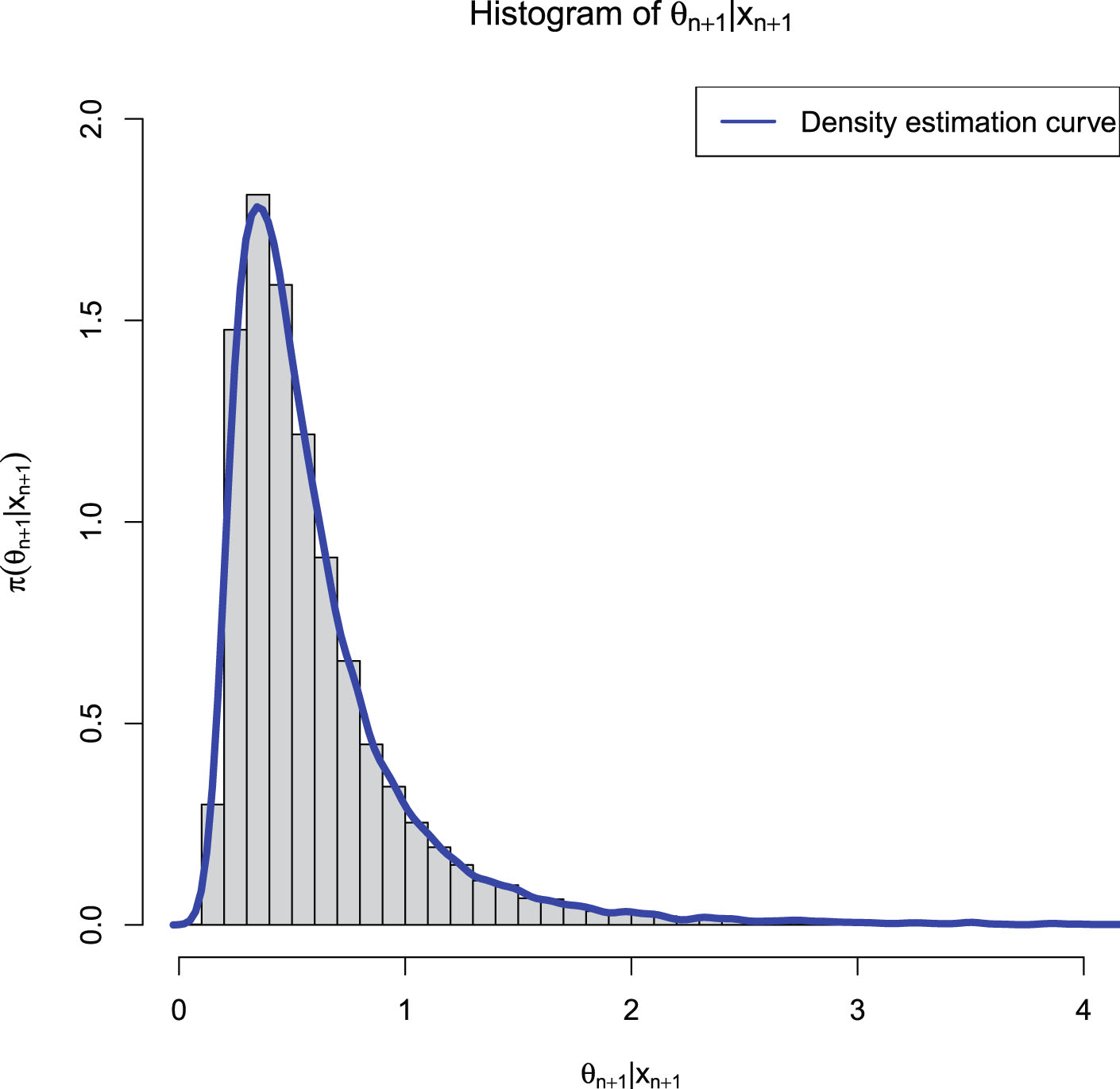
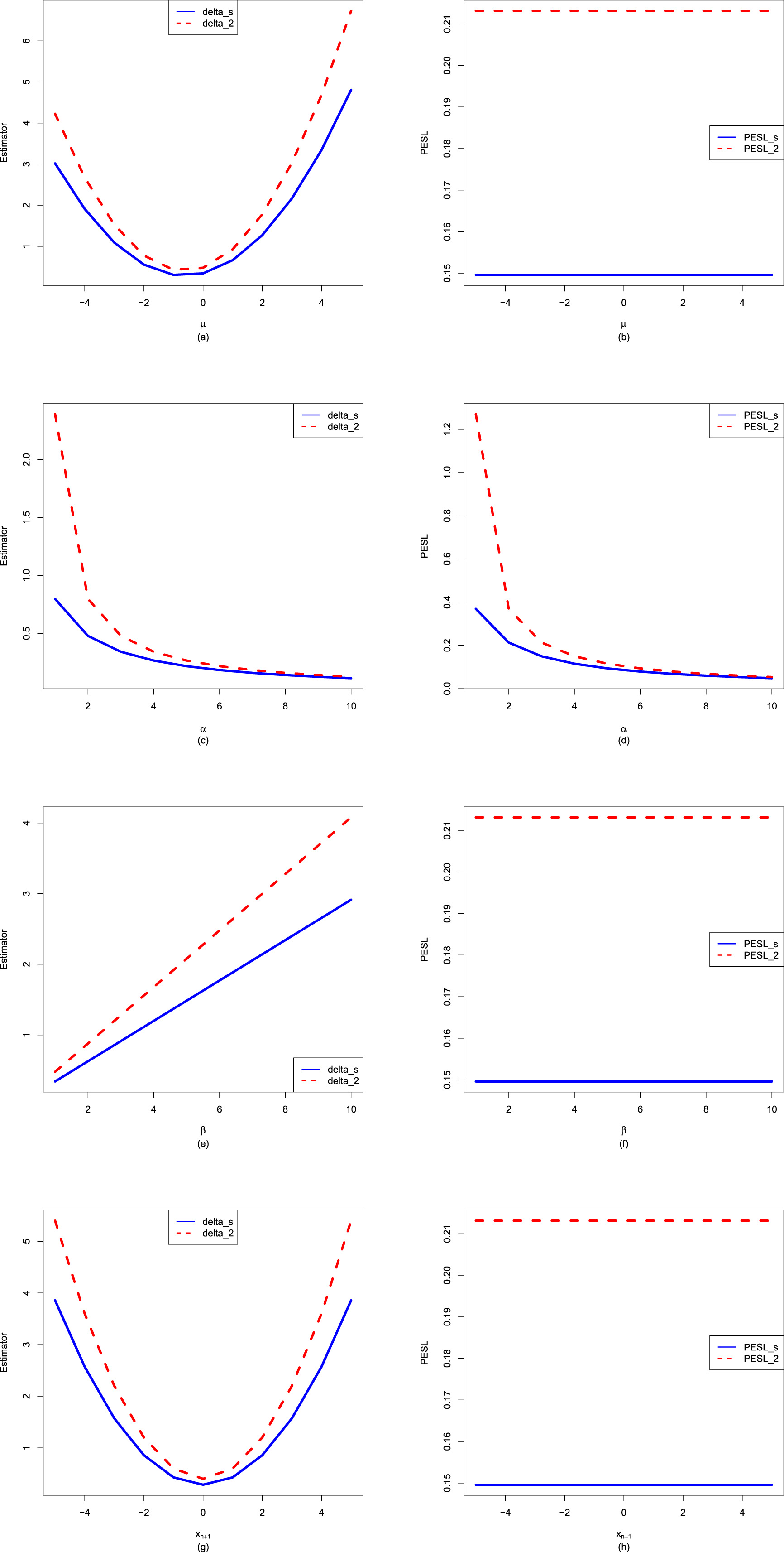
, , , and to change, holding other quantities fixed. In other words, we are interested in the sensitivity analysis of the Bayes estimators and the PESLs about the four quantities , , , and . Figure 5.2 shows the Bayes estimators and the PESLs as functions of , , , and . We see from the left plots of the figure that the Bayes estimators depend on , , , and , and (5.5) is exemplified. Moreover, the Bayes estimators are first decreasing and then increasing functions of , they are decreasing functions of , they are increasing functions of , and they are first decreasing and then increasing functions of . The right plots of the figure exhibit that the PESLs depend only on , but not on , , and , and (5.6) is exemplified. In addition, the PESLs are decreasing functions of . Furthermore, tables 5.1–5.4 display the numerical values of the Bayes estimators and the PESLs in figure 5.2. In summary, the results of figure 5.2 and tables 5.1–5.4 exemplify the two inequalities (5.5) and (5.6).
FIG. 5.1 — N-IG: The histogram of  and the density estimation curve of
  .
.
and the density estimation curve of .
FIG. 5.2 — N-IG: The Bayes estimators and the PESLs as functions of  ,
,  ,
,  , and
, and  . (a), (c), (e), and (g) Bayes estimators vs.
  ,
,  ,
,  , and
, and  . (b), (d), (f), and (h) PESLs vs.
  ,
,  ,
,  , and
, and  .
.
, , , and . (a), (c), (e), and (g) Bayes estimators vs. , , , and . (b), (d), (f), and (h) PESLs vs. , , , and .
TAB. 5.1 — N-IG: The numerical values of the Bayes estimators and the PESLs in figure 5.2:  changes.
changes.
 |
 |
 |
 |
 |
 |
0 | 1 | 2 | 3 | 4 | 5 |
 |
3.0183 | 1.9115 | 1.0905 | 0.5552 | 0.3056 | 0.3418 | 0.6636 | 1.2712 | 2.1645 | 3.3434 | 4.8081 |
 |
4.2256 | 2.6762 | 1.5267 | 0.7773 | 0.4279 | 0.4785 | 0.9291 | 1.7797 | 3.0302 | 4.6808 | 6.7314 |
 |
0.1496 | 0.1496 | 0.1496 | 0.1496 | 0.1496 | 0.1496 | 0.1496 | 0.1496 | 0.1496 | 0.1496 | 0.1496 |
 |
0.2131 | 0.2131 | 0.2131 | 0.2131 | 0.2131 | 0.2131 | 0.2131 | 0.2131 | 0.2131 | 0.2131 | 0.2131 |
TAB. 5.2 — N-IG: The numerical values of the Bayes estimators and the PESLs in figure 5.2:  changes.
changes.
 |
1 | 2 | 3 | 4 | 5 | 6 | 7 | 8 | 9 | 10 |
 |
0.7975 | 0.4785 | 0.3418 | 0.2658 | 0.2175 | 0.1840 | 0.1595 | 0.1407 | 0.1259 | 0.1139 |
 |
2.3924 | 0.7975 | 0.4785 | 0.3418 | 0.2658 | 0.2175 | 0.1840 | 0.1595 | 0.1407 | 0.1259 |
 |
0.3690 | 0.2131 | 0.1496 | 0.1152 | 0.0937 | 0.0789 | 0.0681 | 0.0600 | 0.0536 | 0.0484 |
 |
1.2704 | 0.3690 | 0.2131 | 0.1496 | 0.1152 | 0.0937 | 0.0789 | 0.0681 | 0.0600 | 0.0536 |
TAB. 5.3 — N-IG: The numerical values of the Bayes estimators and the PESLs in figure 5.2:  changes.
changes.
 |
1 | 2 | 3 | 4 | 5 | 6 | 7 | 8 | 9 | 10 |
 |
0.3418 | 0.6275 | 0.9132 | 1.1989 | 1.4846 | 1.7703 | 2.0561 | 2.3418 | 2.6275 | 2.9132 |
 |
0.4785 | 0.8785 | 1.2785 | 1.6785 | 2.0785 | 2.4785 | 2.8785 | 3.2785 | 3.6785 | 4.0785 |
 |
0.1496 | 0.1496 | 0.1496 | 0.1496 | 0.1496 | 0.1496 | 0.1496 | 0.1496 | 0.1496 | 0.1496 |
 |
0.2131 | 0.2131 | 0.2131 | 0.2131 | 0.2131 | 0.2131 | 0.2131 | 0.2131 | 0.2131 | 0.2131 |
TAB. 5.4 — N-IG: The numerical values of the Bayes estimators and the PESLs in figure 5.2:  changes.
changes.
 |
 |
 |
 |
 |
 |
0 | 1 | 2 | 3 | 4 | 5 |
 |
3.8571 | 2.5714 | 1.5714 | 0.8571 | 0.4286 | 0.2857 | 0.4286 | 0.8571 | 1.5714 | 2.5714 | 3.8571 |
 |
5.4000 | 3.6000 | 2.2000 | 1.2000 | 0.6000 | 0.4000 | 0.6000 | 1.2000 | 2.2000 | 3.6000 | 5.4000 |
 |
0.1496 | 0.1496 | 0.1496 | 0.1496 | 0.1496 | 0.1496 | 0.1496 | 0.1496 | 0.1496 | 0.1496 | 0.1496 |
 |
0.2131 | 0.2131 | 0.2131 | 0.2131 | 0.2131 | 0.2131 | 0.2131 | 0.2131 | 0.2131 | 0.2131 | 0.2131 |
Since the Bayes estimators  and
and  and the PESLs
  and
and  depend on
  and
and  , where
  and
and  , we can plot the surfaces of the Bayes estimators and the PESLs on the domain
  via the R function persp3d() in the R package rgl (see Sun et al. (2021); Zhang et al. (2017, 2019b); Adler et al. (2017)). We remark that the R function persp() in the R package graphics can not add another surface to the existing surface, but persp3d() can. Moreover, persp3d() allows one to rotate the perspective plots of the surface according to one’s wishes. Figure 5.3 plots the surfaces of the Bayes estimators and the PESLs, and the surfaces of the differences of the Bayes estimators and the PESLs. The domain for
  is
is  for all the plots. a is for
  and b is for
  in the axes of all the plots. The red surface is for
  and the blue surface is for
  in the upper two plots. From the left two plots of the figure, we see that
  for all
  on
on  . From the right two plots of the figure, we see that
  for all
  on
on  . The results of the figure exemplify the theoretical studies of (5.5) and (5.6).
and and the PESLs and depend on and , where and , we can plot the surfaces of the Bayes estimators and the PESLs on the domain via the R function persp3d() in the R package rgl (see Sun et al. (2021); Zhang et al. (2017, 2019b); Adler et al. (2017)). We remark that the R function persp() in the R package graphics can not add another surface to the existing surface, but persp3d() can. Moreover, persp3d() allows one to rotate the perspective plots of the surface according to one’s wishes. Figure 5.3 plots the surfaces of the Bayes estimators and the PESLs, and the surfaces of the differences of the Bayes estimators and the PESLs. The domain for is for all the plots. a is for and b is for in the axes of all the plots. The red surface is for and the blue surface is for in the upper two plots. From the left two plots of the figure, we see that for all on . From the right two plots of the figure, we see that for all on . The results of the figure exemplify the theoretical studies of (5.5) and (5.6).
5.3.2 Consistencies of the Moment Estimators and the MLEs
In this subsection, similar to subsection 1.8.1, we will numerically exemplify that the moment estimators ( ,
,  , and
, and  ) and the MLEs (
 ,
,  , and
, and  ) are consistent estimators of the hyperparameters (
 ,
,  , and
, and  ) of the hierarchical normal and inverse gamma model (5.1). The motivation of this subsection is that in Theorems 5.2 and 5.3, we have theoretically shown that the moment estimators and the MLEs are consistent estimators of the hyperparameters. Note that only
  are used in this subsection.
, , and ) and the MLEs (, , and ) are consistent estimators of the hyperparameters (, , and ) of the hierarchical normal and inverse gamma model (5.1). The motivation of this subsection is that in Theorems 5.2 and 5.3, we have theoretically shown that the moment estimators and the MLEs are consistent estimators of the hyperparameters. Note that only are used in this subsection.
The frequencies of the moment estimators ( ,
,  , and
, and  ) and the MLEs (
 ,
,  , and
, and  ) of the hyperparameters (
 ,
,  , and
, and  ) as
) as  varies for
  and
and  , 0.5, and 0.1 are reported in table 5.5. From the table, we observe the following facts.
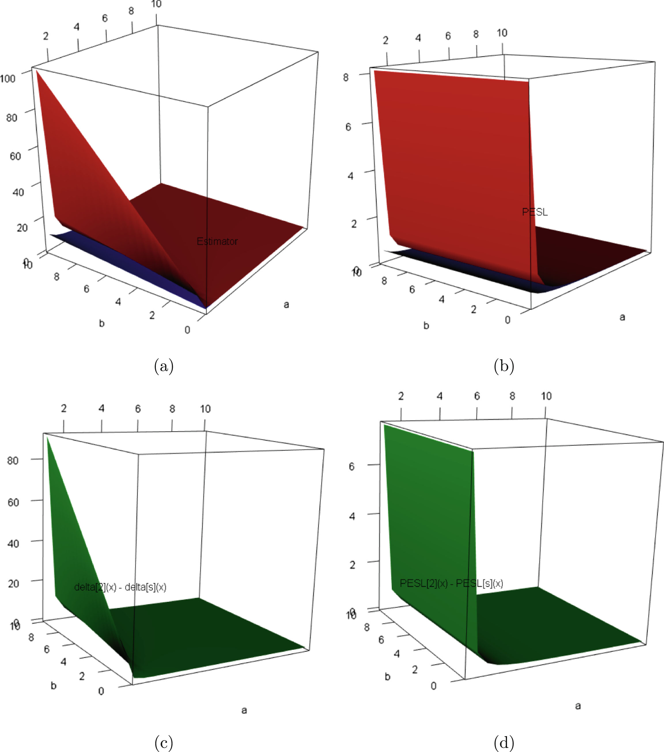
, , and ) and the MLEs (, , and ) of the hyperparameters (, , and ) as varies for and , 0.5, and 0.1 are reported in table 5.5. From the table, we observe the following facts.
FIG. 5.3 — N-IG: (a) The Bayes estimators as functions of  and
and  . (b) The PESLs as functions of
  and
and  . (c) The surface of
  which is positive for all
  on
on  . (d) The surface of
  which is also positive for all
  on
on  .
.
and . (b) The PESLs as functions of and . (c) The surface of which is positive for all on . (d) The surface of which is also positive for all on .
1. Given  , 0.5, or 0.1, the frequencies of the estimators (
 ,
,  ,
,  ,
,  ,
,  ,
,  ) tend to 0 as
  increases to infinity, which means that the moment estimators and the MLEs are consistent estimators of the hyperparameters. For
  , the frequencies of the estimator
  are still very large. However, we observe the tendency to decline to 0 as
  increases to infinity.
, 0.5, or 0.1, the frequencies of the estimators (, , , , , ) tend to 0 as increases to infinity, which means that the moment estimators and the MLEs are consistent estimators of the hyperparameters. For , the frequencies of the estimator are still very large. However, we observe the tendency to decline to 0 as increases to infinity.
2. Comparing the frequencies corresponding to  , 0.5, and 0.1, we observe that as
  gets smaller, the frequencies tend to be larger, since the constraints

, 0.5, and 0.1, we observe that as gets smaller, the frequencies tend to be larger, since the constraints
are easier to meet.
3. Comparing the moment estimators and the MLEs of the hyperparameters  ,
,  , and
, and  , we see that the frequencies of the MLEs are smaller than those of the moment estimators, which means that the MLEs are better than the moment estimators when estimating the hyperparameters in terms of consistency.
, , and , we see that the frequencies of the MLEs are smaller than those of the moment estimators, which means that the MLEs are better than the moment estimators when estimating the hyperparameters in terms of consistency.
5.3.3 Goodness-of-Fit of the Model: KS Test
In this subsection, similar to subsection 1.8.2, we will calculate the goodness-of-fit of the hierarchical normal and inverse gamma model (5.1) to the simulated data. The motivation of this subsection is that we want to check whether the marginal distribution of the hierarchical normal and inverse gamma model (5.1) fits the simulated data well. Note that only  are used in this subsection.
are used in this subsection.
In our problem, the null hypothesis specifies that
 where
where  is the marginal distribution of the hierarchical normal and inverse gamma model (5.1). The marginal density of the
  distribution is given by (5.7) with
  and
and  , which is obviously one-dimensional continuous. Hence, the KS test can be utilized as a measure of the goodness-of-fit.
is the marginal distribution of the hierarchical normal and inverse gamma model (5.1). The marginal density of the distribution is given by (5.7) with and , which is obviously one-dimensional continuous. Hence, the KS test can be utilized as a measure of the goodness-of-fit.
TAB. 5.5 — N-IG: The frequencies of the moment estimators and the MLEs of the hyperparameters as  varies for
  and
and  , 0.5, and 0.1.
varies for and , 0.5, and 0.1.
| Moment estimators | MLEs | ||||||
 |
 |
 |
 |
 |
 |
 |
|
 |
1e4 | 0.00 | 0.00 | 0.00 | 0.00 | 0.00 | 0.00 |
| 2e4 | 0.00 | 0.00 | 0.00 | 0.00 | 0.00 | 0.00 | |
| 4e4 | 0.00 | 0.00 | 0.00 | 0.00 | 0.00 | 0.00 | |
| 8e4 | 0.00 | 0.00 | 0.00 | 0.00 | 0.00 | 0.00 | |
| 16e4 | 0.00 | 0.00 | 0.00 | 0.00 | 0.00 | 0.00 | |
| 32e4 | 0.00 | 0.00 | 0.00 | 0.00 | 0.00 | 0.00 | |
 |
1e4 | 0.00 | 0.19 | 0.00 | 0.00 | 0.02 | 0.00 |
| 2e4 | 0.00 | 0.09 | 0.00 | 0.00 | 0.00 | 0.00 | |
| 4e4 | 0.00 | 0.04 | 0.00 | 0.00 | 0.00 | 0.00 | |
| 8e4 | 0.00 | 0.00 | 0.00 | 0.00 | 0.00 | 0.00 | |
| 16e4 | 0.00 | 0.00 | 0.00 | 0.00 | 0.00 | 0.00 | |
| 32e4 | 0.00 | 0.01 | 0.00 | 0.00 | 0.00 | 0.00 | |
 |
1e4 | 0.00 | 0.80 | 0.61 | 0.00 | 0.56 | 0.22 |
| 2e4 | 0.00 | 0.81 | 0.49 | 0.00 | 0.42 | 0.07 | |
| 4e4 | 0.00 | 0.67 | 0.37 | 0.00 | 0.33 | 0.00 | |
| 8e4 | 0.00 | 0.55 | 0.21 | 0.00 | 0.08 | 0.00 | |
| 16e4 | 0.00 | 0.48 | 0.12 | 0.00 | 0.01 | 0.00 | |
| 32e4 | 0.00 | 0.39 | 0.07 | 0.00 | 0.00 | 0.00 | |
The results of the KS test goodness-of-fit of the model (5.1) to the simulated data are reported in table 5.6. Note that the data are simulated according to the hierarchical normal and inverse gamma model (5.1) with  ,
,  , and
, and  . In the table, the hyperparameters
  ,
,  , and
, and  are estimated by three methods. The first method is the oracle method, in that we know the hyperparameters
  ,
,  , and
, and  . The second method is the moment method, in that the hyperparameters
  ,
,  , and
, and  are estimated by their moment estimators (see Theorem 5.2). The third method is the MLE method, in that the hyperparameters
  ,
,  , and
, and  are estimated by their MLEs (see Theorem 5.3). In the table, the sample size is
  , and the number of simulations is
  .
.
, , and . In the table, the hyperparameters , , and are estimated by three methods. The first method is the oracle method, in that we know the hyperparameters , , and . The second method is the moment method, in that the hyperparameters , , and are estimated by their moment estimators (see Theorem 5.2). The third method is the MLE method, in that the hyperparameters , , and are estimated by their MLEs (see Theorem 5.3). In the table, the sample size is , and the number of simulations is .
From table 5.6, we observe the following facts.
1. The  values for the three methods are respectively given by 0.0267, 0.0226, and 0.0199, which means that the MLE method is the best method, the moment method is the second-best method, and the oracle method is the worst method. A possible explanation for this phenomenon is that in (1.23), the empirical cdf
  is based on data, and the population cdfs
  for the MLE method and the moment method are also based on data, while the population cdf
  for the oracle method is not based on data.
values for the three methods are respectively given by 0.0267, 0.0226, and 0.0199, which means that the MLE method is the best method, the moment method is the second-best method, and the oracle method is the worst method. A possible explanation for this phenomenon is that in (1.23), the empirical cdf is based on data, and the population cdfs for the MLE method and the moment method are also based on data, while the population cdf for the oracle method is not based on data.
2. The  values for the three methods are respectively given by 0.5207, 0.6772, and 0.7832, which also means that the MLE method ranks first, the moment method ranks second, and the oracle method ranks third. The possible explanation for this phenomenon is described in the previous paragraph.
values for the three methods are respectively given by 0.5207, 0.6772, and 0.7832, which also means that the MLE method ranks first, the moment method ranks second, and the oracle method ranks third. The possible explanation for this phenomenon is described in the previous paragraph.
3. The  values for the three methods are respectively given by 0.14, 0.26, and 0.60. The
  value for the MLE method accounts for over half of the
  simulations. The order of preference for the three methods is the MLE method, the moment method, and the oracle method.
values for the three methods are respectively given by 0.14, 0.26, and 0.60. The value for the MLE method accounts for over half of the simulations. The order of preference for the three methods is the MLE method, the moment method, and the oracle method.
4. The  values for the three methods are respectively given by 0.14, 0.26, and 0.60. A small
  value corresponds to a large p-value. Hence, the smallest
  value corresponds to the largest p-value. Therefore, the
  value and the
  value for the three methods are the same. The order of preference for the three methods is the MLE method, the moment method, and the oracle method.
values for the three methods are respectively given by 0.14, 0.26, and 0.60. A small value corresponds to a large p-value. Hence, the smallest value corresponds to the largest p-value. Therefore, the value and the value for the three methods are the same. The order of preference for the three methods is the MLE method, the moment method, and the oracle method.
5. The  values for the three methods are respectively given by
  ,
,  , and
, and  . The
. The  values for the three methods are nearly
  , which means that the three methods have good performances in terms of goodness-of-fit.
values for the three methods are respectively given by , , and . The values for the three methods are nearly , which means that the three methods have good performances in terms of goodness-of-fit.
6. In summary, for the five indices ( ,
,  ,
,  ,
,  ,
,  ), the order of preference for the three methods is the MLE method, the moment method, and the oracle method. Comparing the moment method and the MLE method, we find that the MLE method has a better performance than the moment method in terms of all five indices.
, , , , ), the order of preference for the three methods is the MLE method, the moment method, and the oracle method. Comparing the moment method and the MLE method, we find that the MLE method has a better performance than the moment method in terms of all five indices.
The boxplots of the  values and the p-values for the three methods are displayed in figure 5.4. From the figure, we observe the following facts.
values and the p-values for the three methods are displayed in figure 5.4. From the figure, we observe the following facts.
TAB. 5.6 — N-IG: The results of the KS test goodness-of-fit of the model (5.1) to the simulated data.
 |
 |
 |
|
 |
0.0267 | 0.0226 | 0.0199 |
 |
0.5207 | 0.6772 | 0.7832 |
 |
0.14 | 0.26 | 0.60 |
 |
0.14 | 0.26 | 0.60 |
 |
0.98 | 1.00 | 1.00 |
1. The  values of the oracle method are larger than those of the other two methods. Since for the
  value, the smaller the better, the order of preference for the three methods is the MLE method, the moment method, and the oracle method.
values of the oracle method are larger than those of the other two methods. Since for the value, the smaller the better, the order of preference for the three methods is the MLE method, the moment method, and the oracle method.
2. The p-values of the oracle method are smaller than those of the other two methods. Since for the p-value, the larger the better, the order of preference for the three methods is the MLE method, the moment method, and the oracle method.
3. Small  values correspond to large p-values, and large
  values correspond to small p-values.
values correspond to large p-values, and large values correspond to small p-values.
4. The MLE method has a better performance than the moment method in terms of the  values and the p-values.
values and the p-values.
5.3.4 Numerical Comparisons of the Bayes Estimators and the PESLs of Three Methods
In this subsection, we will numerically compare the Bayes estimators and the PESLs of the three methods (the oracle method, the moment method, and the MLE method). The motivation of this subsection is that the theoretical comparisons of the Bayes estimators and the PESLs of the three methods can be found in subsection 5.2.3. Note that the full data  are used in this subsection.
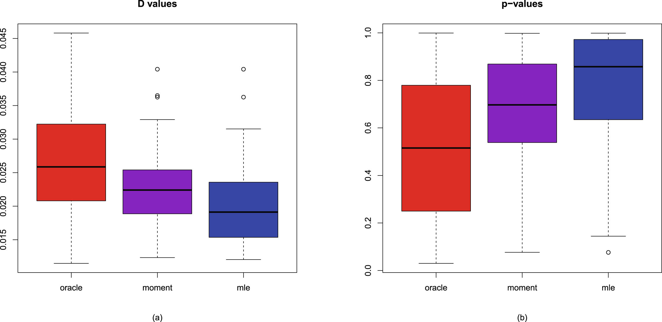
are used in this subsection.
FIG. 5.4 — N-IG: The boxplots of the  values and the p-values for the three methods. (a)
  values. (b) p-values.
values and the p-values for the three methods. (a) values. (b) p-values.
Note that the data are simulated according to the hierarchical normal and inverse gamma model (5.1) with the hyperparameters specified by  ,
,  , and
, and  . Moreover, the oracle method knows the hyperparameters
  ,
,  , and
, and  in simulations.
, , and . Moreover, the oracle method knows the hyperparameters , , and in simulations.
Comparisons of the Bayes estimators and the PESLs of the three methods for sample size  and number of simulations
  are displayed in figure 5.5. From the figure, we observe the following facts.
and number of simulations are displayed in figure 5.5. From the figure, we observe the following facts.
1. For the estimators of  , the MLE method is slightly closer to the oracle method than the moment method.
, the MLE method is slightly closer to the oracle method than the moment method.
2. For the estimators of  and
and  , the MLE method is much closer to the oracle method than the moment method.
and , the MLE method is much closer to the oracle method than the moment method.
3. For the Bayes estimators  and
and 
 , the MLE method is slightly closer to the oracle method than the moment method.
and , the MLE method is slightly closer to the oracle method than the moment method.
4. For the PESLs  and
and 
 , the MLE method is much closer to the oracle method than the moment method.
and , the MLE method is much closer to the oracle method than the moment method.
5. All the plots indicate that the MLE method is better than the moment method, as the estimators of the hyperparameters, the Bayes estimators, and the PESLs of the MLE method are closer to those of the oracle method than those of the moment method.
The boxplots of the absolute errors from the oracle method by the moment method and the MLE method for sample size  and number of simulations
  are displayed in figure 5.6. All the plots indicate that the MLE method is better than the moment method, as the absolute errors from the oracle method of the estimators of the hyperparameters, the Bayes estimators, and the PESLs by the MLE method are much smaller than those of the moment method.
and number of simulations are displayed in figure 5.6. All the plots indicate that the MLE method is better than the moment method, as the absolute errors from the oracle method of the estimators of the hyperparameters, the Bayes estimators, and the PESLs by the MLE method are much smaller than those of the moment method.
The averages and proportions of the absolute errors from the oracle method by the moment method and the MLE method for the estimators of the hyperparameters, the Bayes estimators, and the PESLs are summarized in table 5.7. See subsection 1.8.3 for details. From the table, we observe that the averages of the absolute errors from the oracle method by the MLE method are much smaller than those from the moment method. Moreover, the proportions of the absolute errors from the oracle method by the MLE method are much larger than those by the moment method. In summary, the table illustrates that the MLE method is better than the moment method in terms of the averages and proportions of the absolute errors from the oracle method.
The MSE, MAE, and MEE of the estimators of the hyperparameters by the moment method and the MLE method are summarized in table 5.8. See subsection 1.8.3 for details. From the table, we see that the MLE method is slightly better than the moment method when estimating the hyperparameter  , as the MSE and MAE of the MLE method are slightly smaller than those of the moment method. Moreover, the MLE method is far better than the moment method when estimating the hyperparameters
  and
and  , as the MSE, MAE, and MEE of the MLE method are much smaller than those of the moment method. Note that in the table, there are two NaNs for the MEE when estimating the hyperparameter
  , because the entropy (or Stein’s) loss function only applies to a positive parameter, but now
  and thus the entropy loss function does not apply.
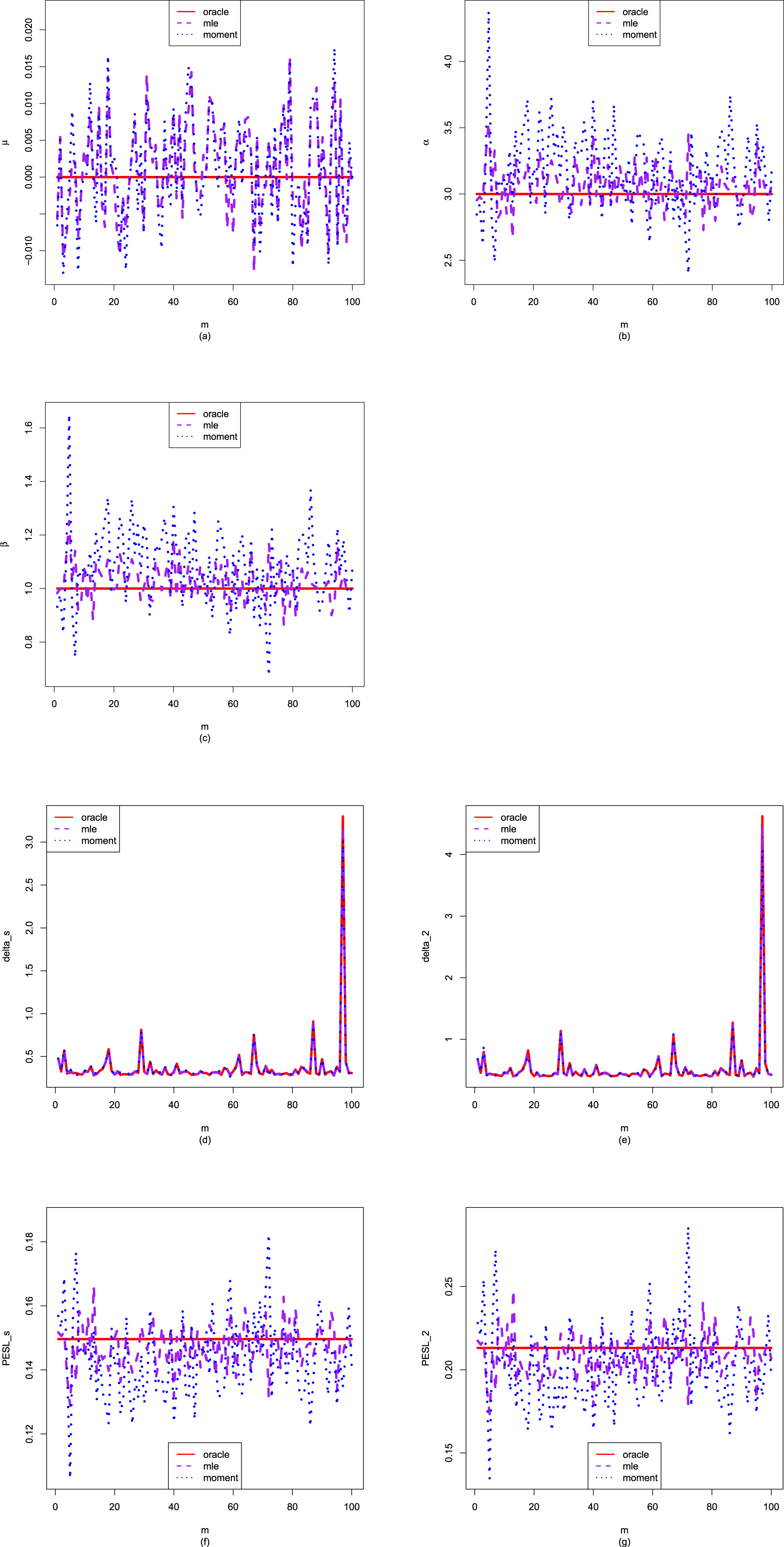
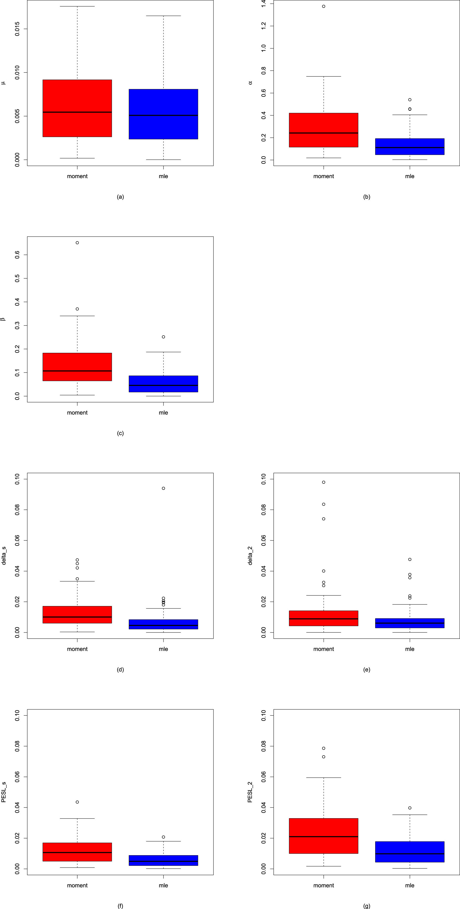
, as the MSE and MAE of the MLE method are slightly smaller than those of the moment method. Moreover, the MLE method is far better than the moment method when estimating the hyperparameters and , as the MSE, MAE, and MEE of the MLE method are much smaller than those of the moment method. Note that in the table, there are two NaNs for the MEE when estimating the hyperparameter , because the entropy (or Stein’s) loss function only applies to a positive parameter, but now and thus the entropy loss function does not apply.
FIG. 5.5 — N-IG: Comparisons of  ,
,  ,
,  ,
,  ,
,  ,
,  , and
, and  of the three methods for sample size
  and number of simulations
  . (a)
. (a)  . (b)
. (b)  . (c)
. (c)  . (d)
. (d)  . (e)
. (e)  . (f)
. (f)  . (g)
. (g)  .
.
, , , , , , and of the three methods for sample size and number of simulations . (a) . (b) . (c) . (d) . (e) . (f) . (g) .
FIG. 5.6 — N-IG: The boxplots of the absolute errors from the oracle method by the moment method and the MLE method for sample size  and number of simulations
  . (a)
. (a)  . (b)
. (b)  . (c)
. (c)  . (d)
. (d)  . (e)
. (e)  . (f)
. (f)  . (g)
. (g)  .
.
and number of simulations . (a) . (b) . (c) . (d) . (e) . (f) . (g) .
TAB. 5.7 — N-IG: The averages and proportions of the absolute errors from the oracle method by the moment method and the MLE method for the estimators of the hyperparameters, the Bayes estimators, and the PESLs.
| Averages | Proportions | |||
| Moment | MLE | Moment | MLE | |
 |
0.0060 | 0.0055 | 0.46 | 0.54 |
 |
0.2852 | 0.1350 | 0.21 | 0.79 |
 |
0.1349 | 0.0563 | 0.21 | 0.79 |
 |
0.0147 | 0.0067 | 0.23 | 0.77 |
 |
0.0172 | 0.0093 | 0.36 | 0.64 |
 |
0.0117 | 0.0058 | 0.21 | 0.79 |
 |
0.0231 | 0.0116 | 0.21 | 0.79 |
TAB. 5.8 — N-IG: The MSE, MAE, and MEE of the estimators of the hyperparameters by the moment method and the MLE method.
| MSE | MAE | MEE | ||||
| Moment | MLE | Moment | MLE | Moment | MLE | |
 |
0.00005 | 0.00004 | 0.00598 | 0.00554 | NaN | NaN |
 |
0.12745 | 0.03044 | 0.28523 | 0.13502 | 0.00642 | 0.00162 |
 |
0.02790 | 0.00552 | 0.13486 | 0.05634 | 0.01237 | 0.00262 |
5.3.5 Marginal Densities for Various Hyperparameters
In this subsection, we will plot the marginal densities of the hierarchical normal and inverse gamma model (5.1) for various hyperparameters  ,
,  , and
, and  . The motivation of this subsection is that we want to know what kind of data can be modeled by the hierarchical normal and inverse gamma model (5.1). Note that the marginal density of
  is given by (5.7) specified by three hyperparameters
  ,
,  , and
, and  . We will explore how the marginal densities change around the marginal density with hyperparameters specified by
  ,
,  , and
, and  . Other numerical values of the hyperparameters can also be specified.
, , and . The motivation of this subsection is that we want to know what kind of data can be modeled by the hierarchical normal and inverse gamma model (5.1). Note that the marginal density of is given by (5.7) specified by three hyperparameters , , and . We will explore how the marginal densities change around the marginal density with hyperparameters specified by , , and . Other numerical values of the hyperparameters can also be specified.
Figure 5.7 plots the marginal densities for varied  , holding
  and
and  fixed. From the figure, we see that as
  increases, the marginal density shifts to the right, while keeping the shape of the curve unchanged. That is,
  is a location parameter. Moreover, all the marginal densities are symmetric about the mean
  .
.
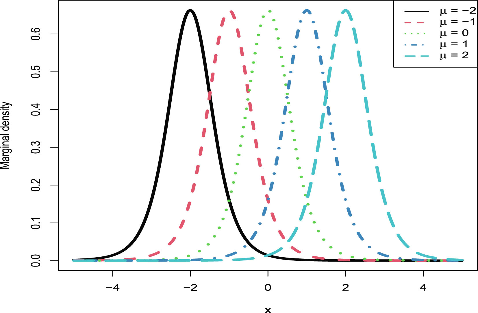
, holding and fixed. From the figure, we see that as increases, the marginal density shifts to the right, while keeping the shape of the curve unchanged. That is, is a location parameter. Moreover, all the marginal densities are symmetric about the mean .
FIG. 5.7 — N-IG: The marginal densities for varied  , holding
  and
and  fixed.
, holding and fixed.
Figure 5.8 plots the marginal densities for varied  , holding
  and
and  fixed. From the figure, we see that as
  increases, the peak value of the curve also increases. In other words, the variance of the marginal distribution decreases, as
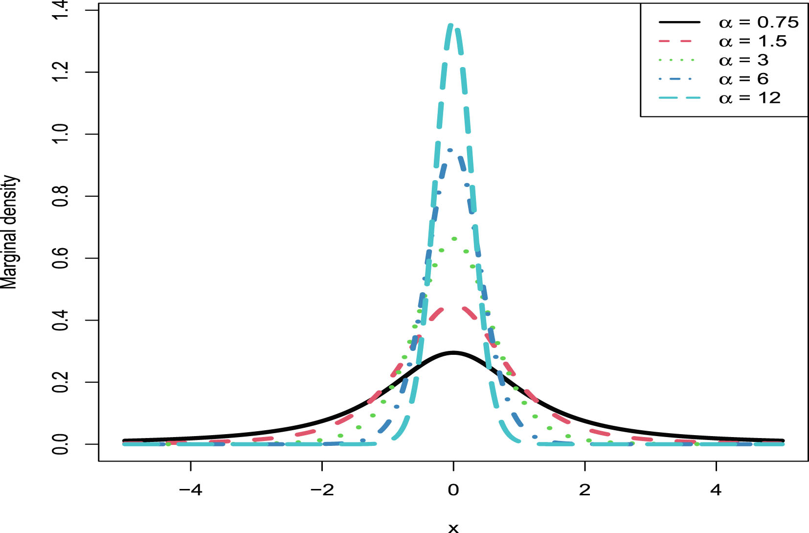
 (5.14)
is a decreasing function of
(5.14)
is a decreasing function of  . Moreover, all the marginal densities are symmetric about the mean
  .
.
, holding and fixed. From the figure, we see that as increases, the peak value of the curve also increases. In other words, the variance of the marginal distribution decreases, as
FIG. 5.8 — N-IG: The marginal densities for varied  , holding
  and
and  fixed.
, holding and fixed.
(5.14)
. Moreover, all the marginal densities are symmetric about the mean .
Figure 5.9 plots the marginal densities for varied  , holding
  and
and  fixed. From the figure, we see that as
  increases, the peak value of the curve decreases. In other words, the variance of the marginal distribution increases, as
  given by (5.14) is an increasing function of
  . Moreover, all the marginal densities are symmetric about the mean
  .
.
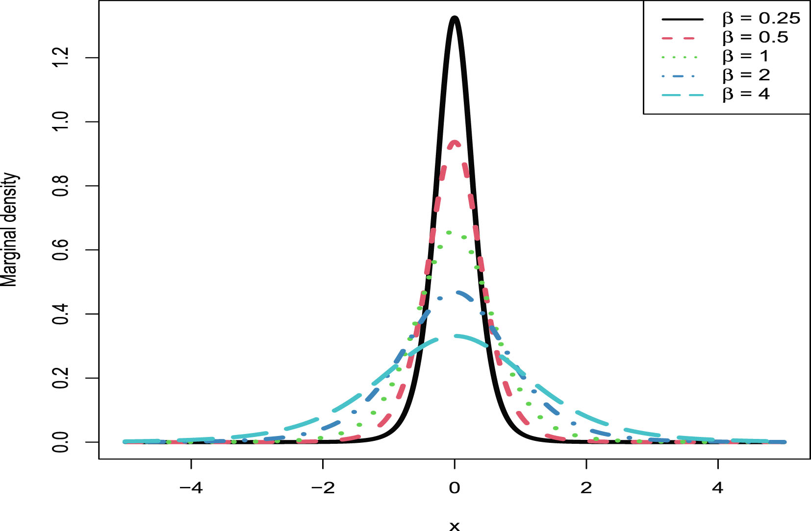
, holding and fixed. From the figure, we see that as increases, the peak value of the curve decreases. In other words, the variance of the marginal distribution increases, as given by (5.14) is an increasing function of . Moreover, all the marginal densities are symmetric about the mean .
FIG. 5.9 — N-IG: The marginal densities for varied  , holding
  and
and  fixed.
, holding and fixed.
5.4 A Real Data Example
In this section, we utilize the percentage of body fat data of 250  men of various ages to illustrate our methods (see DASL (Data And Story Library) (2019)). The percentage of body fat is the percentage of a person’s body that is fat, which is a matter of concern for health and fitness.
men of various ages to illustrate our methods (see DASL (Data And Story Library) (2019)). The percentage of body fat is the percentage of a person’s body that is fat, which is a matter of concern for health and fitness.
The histogram of the sample  (the percentage of body fat data) along with its density estimation curve, are depicted in figure 5.10. From the figure, we see that the density estimation curve is roughly bell-shaped and symmetric around its mean, and thus the hierarchical normal and inverse gamma model (5.1) should be appropriate. See subsection “Marginal densities for various hyperparameters” for details.
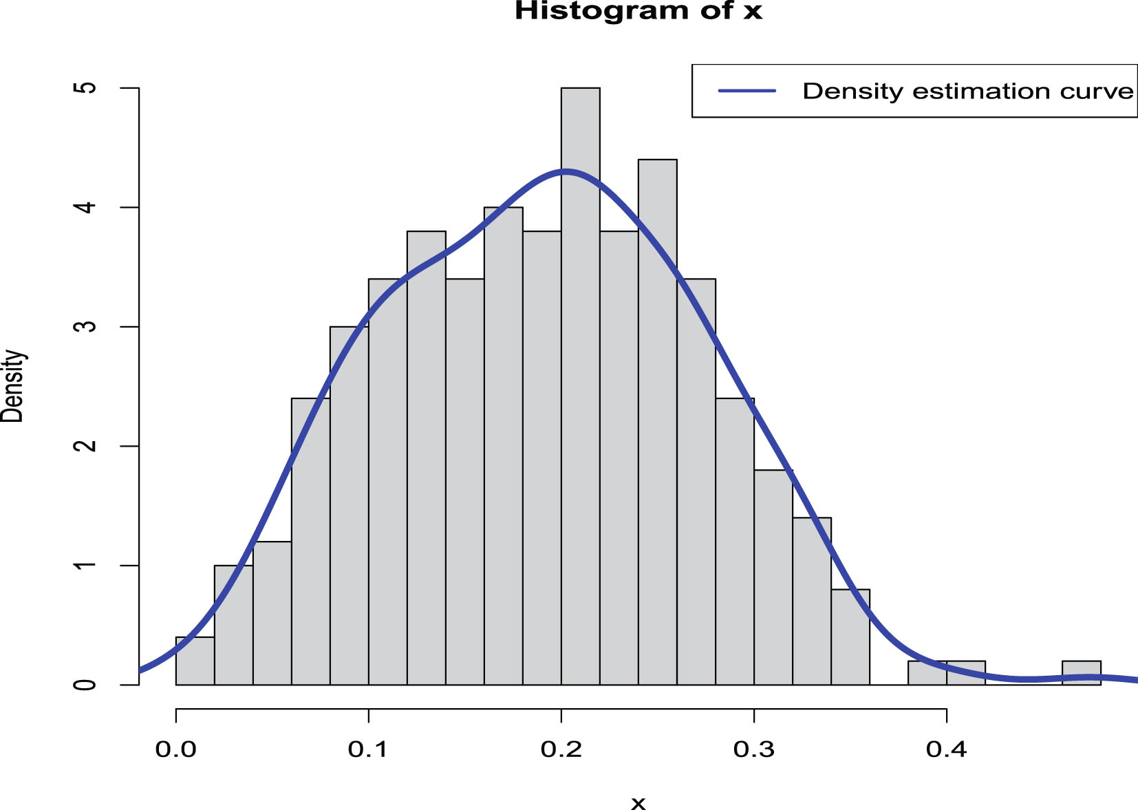
(the percentage of body fat data) along with its density estimation curve, are depicted in figure 5.10. From the figure, we see that the density estimation curve is roughly bell-shaped and symmetric around its mean, and thus the hierarchical normal and inverse gamma model (5.1) should be appropriate. See subsection “Marginal densities for various hyperparameters” for details.
FIG. 5.10 — N-IG: The histogram of the sample  along with its density estimation curve.
along with its density estimation curve.
The estimators of the hyperparameters  ,
,  , and
, and  , the goodness-of-fit of the model, the empirical Bayes estimators of the variance parameter of the normal distribution with a conjugate inverse gamma prior and the PESLs, and the mean and variance of the percentage of body fat data by the moment method and the MLE method are summarized in table 5.9. From the table, we observe the following facts.
, , and , the goodness-of-fit of the model, the empirical Bayes estimators of the variance parameter of the normal distribution with a conjugate inverse gamma prior and the PESLs, and the mean and variance of the percentage of body fat data by the moment method and the MLE method are summarized in table 5.9. From the table, we observe the following facts.
1. The moment estimator of the hyperparameter  is equal to the sample mean
  of the first
  observations. It is interesting to note that the MLE of the hyperparameter
  is equal to 0.1897987, which is very similar to the moment estimator of the hyperparameter
  . But the moment estimators and the MLEs of the hyperparameters
  and
and  are quite different. This does not mean that the hierarchical normal and inverse gamma model (5.1) does not fit the real data, nor mean that the moment estimators and the MLEs are not consistent estimators of the hyperparameters
  and
and  . The reason for the big differences between the two estimators is that the sample size
  is too small. Of course, the MLEs of the hyperparameters
  and
and  are more reliable, as assured from the previous figures and tables in the simulations section.
is equal to the sample mean of the first observations. It is interesting to note that the MLE of the hyperparameter is equal to 0.1897987, which is very similar to the moment estimator of the hyperparameter . But the moment estimators and the MLEs of the hyperparameters and are quite different. This does not mean that the hierarchical normal and inverse gamma model (5.1) does not fit the real data, nor mean that the moment estimators and the MLEs are not consistent estimators of the hyperparameters and . The reason for the big differences between the two estimators is that the sample size is too small. Of course, the MLEs of the hyperparameters and are more reliable, as assured from the previous figures and tables in the simulations section.
2. We use the KS test as a measure of the goodness-of-fit. The p-value of the moment method is  , and thus the
  distribution with
  ,
,  , and
, and  estimated by their moment estimators fits the sample
  well. Moreover, the p-value of the MLE method is
  , and thus the
  distribution with
  ,
,  , and
, and  estimated by their MLEs fits the sample
  even better. When comparing the two methods, we observe that the
  value of the MLEs is smaller, and the p-value of the MLEs is larger, which means that the
  distribution with the hyperparameters
  ,
,  , and
, and  estimated by the MLEs has a better fit to the sample
  than that estimated by the moment estimators.
, and thus the distribution with , , and estimated by their moment estimators fits the sample well. Moreover, the p-value of the MLE method is , and thus the distribution with , , and estimated by their MLEs fits the sample even better. When comparing the two methods, we observe that the value of the MLEs is smaller, and the p-value of the MLEs is larger, which means that the distribution with the hyperparameters , , and estimated by the MLEs has a better fit to the sample than that estimated by the moment estimators.
3. When the hyperparameters are estimated by the MLE method, we see that
 and
and

When the hyperparameters are estimated by the moment method, we observe a similar phenomenon for the Bayes estimators and the PESLs. Consequently, the two inequalities (5.5) and (5.6) are exemplified.
4. The mean of  (the percentage of body fat data) is estimated by
  . By (5.14), the variance of
  is estimated by
  . It is interesting to note that the mean and variance of
  by the two methods are very similar, although the estimators of the hyperparameters are quite different. Moreover, it is worthy to mention that
 for the MLE method. The mean and variance of
  are similar for the moment method. Therefore, the variance of
  is quite small, not large!
(the percentage of body fat data) is estimated by . By (5.14), the variance of is estimated by . It is interesting to note that the mean and variance of by the two methods are very similar, although the estimators of the hyperparameters are quite different. Moreover, it is worthy to mention that
are similar for the moment method. Therefore, the variance of is quite small, not large!
TAB. 5.9 — N-IG: The estimators of the hyperparameters, the goodness-of-fit of the model, the empirical Bayes estimators of the variance parameter of the normal distribution and the PESLs, and the mean and variance of the percentage of bodyfat data by the moment method and the MLE method.
| Moment method | MLE method | ||
| Estimators of the hyperparameters |  |
 |
 |
 |
 |
 |
|
 |
 |
 |
|
| Goodness-of-fit of the model |  |
0.0618 | 0.0449 |
| p-value | 0.2968 | 0.6983 | |
| Empirical Bayes estimators and PESLs |  |
0.0064531 | 0.0068121 |
 |
0.0079852 | 0.0068128 | |
 |
0.0989905 | 5.2824e-05 | |
 |
0.1233821 | 5.2829e-05 | |
| Mean and variance of the percentage of body fat data |  |
0.1897992 | 0.1897987 |
 |
0.006812273 | 0.006812272 |
5.5 Conclusions and Discussions
For the hierarchical normal and inverse gamma model (5.1), we calculate the posterior distribution of  ,
,  , in Theorem 5.1. After that, we calculate the Bayes estimators of
  ,
,  and
and  , and the PESLs of
  ,
,  and
and  . Moreover, they satisfy two inequalities (5.5) and (5.6). After proving some lemmas, the estimators of the hyperparameters of the model (5.1) by the moment method and their consistencies are summarized in Theorem 5.2. Furthermore, the estimators of the hyperparameters of the model (5.1) by the MLE method and their consistencies are summarized in Theorem 5.3. Finally, the empirical Bayes estimators of the variance parameter of the model (5.1) under Stein’s loss function by the moment method and the MLE method are summarized in Theorem 5.4.
, , in Theorem 5.1. After that, we calculate the Bayes estimators of , and , and the PESLs of , and . Moreover, they satisfy two inequalities (5.5) and (5.6). After proving some lemmas, the estimators of the hyperparameters of the model (5.1) by the moment method and their consistencies are summarized in Theorem 5.2. Furthermore, the estimators of the hyperparameters of the model (5.1) by the MLE method and their consistencies are summarized in Theorem 5.3. Finally, the empirical Bayes estimators of the variance parameter of the model (5.1) under Stein’s loss function by the moment method and the MLE method are summarized in Theorem 5.4.
In the simulations section, we have illustrated five aspects. First, we have numerically exemplified two inequalities of the Bayes estimators and the PESLs (5.5) and (5.6). Second, we have illustrated that the moment estimators and the MLEs are consistent estimators of the hyperparameters. Third, we have calculated the goodness-of-fit of the model to the simulated data. Fourth, we have numerically compared the Bayes estimators and the PESLs of the three methods. Finally, we have plotted the marginal densities of the model for various hyperparameters.
Note that in Theorem 5.3, we only stated that the estimators of the hyperparameters of the model (5.1) by the MLE method  ,
,  , and
, and  are the solutions to the equations (5.11)–(5.13). We can exploit Newton’s method to solve the equations (5.11)–(5.13) and to numerically obtain the MLEs of
  ,
,  , and
, and  . However, we can not prove the existence and uniqueness of the solutions to our system. The interested readers who have such kind of knowledge and skills are encouraged to solve this issue.
, , and are the solutions to the equations (5.11)–(5.13). We can exploit Newton’s method to solve the equations (5.11)–(5.13) and to numerically obtain the MLEs of , , and . However, we can not prove the existence and uniqueness of the solutions to our system. The interested readers who have such kind of knowledge and skills are encouraged to solve this issue.
We utilize the percentage of body fat data of 250 men of various ages to illustrate our methods. The estimators of the hyperparameters  ,
,  , and
, and  , the goodness-of-fit of the model, the empirical Bayes estimators of the variance parameter of the normal distribution with a conjugate inverse gamma prior and the PESLs, and the mean and variance of the percentage of body fat data by the moment method and the MLE method are summarized in table 5.9. The
  distribution with the hyperparameters
  ,
,  , and
, and  estimated by the MLEs has a better goodness-of-fit to the sample
  than that estimated by the moment estimators. Moreover, the two inequalities (5.5) and (5.6) are exemplified for the sample
  .
.
, , and , the goodness-of-fit of the model, the empirical Bayes estimators of the variance parameter of the normal distribution with a conjugate inverse gamma prior and the PESLs, and the mean and variance of the percentage of body fat data by the moment method and the MLE method are summarized in table 5.9. The distribution with the hyperparameters , , and estimated by the MLEs has a better goodness-of-fit to the sample than that estimated by the moment estimators. Moreover, the two inequalities (5.5) and (5.6) are exemplified for the sample .
From Lemma 5.3, we see that the data from the non-standardized Student-t distribution should have a good goodness-of-fit of the hierarchical normal and inverse gamma model.
Comparing the two Bayes estimators  and
and  of the variance parameter
  , we prefer Stein’s estimator
  , not because it is larger or smaller than the squared error estimator
  , but because Stein’s loss function is more appropriate than the squared error loss function for the positive parameter
  . Note that Stein’s loss function penalizes gross overestimation and gross underestimation equally for
  , but the squared error loss function does not.
and of the variance parameter , we prefer Stein’s estimator , not because it is larger or smaller than the squared error estimator , but because Stein’s loss function is more appropriate than the squared error loss function for the positive parameter . Note that Stein’s loss function penalizes gross overestimation and gross underestimation equally for , but the squared error loss function does not.
For the hierarchical normal and inverse gamma model (5.1), we can calculate the estimators of the hyperparameters, since the marginal distribution of the model (5.1) is proper. In empirical Bayes analysis, we use the marginal distribution to estimate the hyperparameters from the observations. There are two frequently used methods to estimate the hyperparameters by utilizing the marginal distribution, i.e., the moment method and the MLE method. In this chapter, we use the two methods to estimate the hyperparameters of the hierarchical normal and inverse gamma model (5.1).
Now we present some future work. One may consider extending the hierarchical normal and inverse gamma model (5.1) to different types of non-conjugate priors for the variance parameter of the normal distribution (see Berger et al. (2015); Berger (1985) and the references therein). In these situations, one may not obtain analytical solutions; then one should be able to derive the estimators numerically.
Chapter 6 The Empirical Bayes Estimators of the Variance Parameter of the Normal Distribution with a Normal-Inverse-Gamma Prior under Stein’s Loss Function
For the hierarchical normal and normal-inverse-gamma model, we calculate the Bayes estimator of the variance parameter of the normal distribution under Stein’s loss function, which penalizes gross overestimation and gross underestimation equally and the corresponding PESL. We also obtain the Bayes estimator of the variance parameter under the squared error loss function and the corresponding PESL. Moreover, we obtain the empirical Bayes estimators of the variance parameter of the normal distribution with a conjugate normal-inverse-gamma prior by the moment method and the MLE method. In numerical simulations, we have illustrated four aspects: The two inequalities of the Bayes estimators and the PESLs; the consistencies of the moment estimators and the MLEs of the hyperparameters; the goodness-of-fit of the model to the simulated data; and the plots of the marginal densities for various hyperparameters. The numerical results indicate that the MLEs are better than the moment estimators when estimating the hyperparameters. Finally, we utilize the poverty level data, which represent percentages of all persons below the poverty level, to illustrate our theoretical studies.
Acknowledgement. This chapter is derived in part from an article Zhang (2025) under review in the Chinese Journal of Applied Probability and Statistics and an article Zhang et al. (2019a) published in Communications in Statistics-Theory and Methods 01 February 2019 <copyright Taylor & Francis>, available online: http://www.tandfonline.com/10.1080/03610926.2018.1465081.
6.1 Introduction
The motivations of this chapter are summarized as follows. Example 1.5.1 (p. 20) of Mao and Tang (2012), part I (pp. 69–70) of Chen (2014), and Zhang et al. (2019a) have considered the following hierarchical normal and normal-inverse-gamma model:
 (6.1)
where
(6.1)
where  ,
,  ,
,  , and
, and  are known hyperparameters, and iid means independent and identically distributed. The
  distribution is a joint conjugate prior for
  of the normal distribution
  , so that the posterior distribution of
  is an
is an  distribution with updated hyperparameters. However, in reality, the hyperparameters are unknown. Zhang et al. (2019a) have estimated the hyperparameters of the model (6.1) by the moment method and the MLE method. Moreover, they obtained the Bayes estimators of the mean and variance parameters of the model (6.1) under the squared error loss function. Finally, they obtained the empirical Bayes estimators of the mean and variance parameters of the model (6.1) under the squared error loss function by the moment method and the MLE method. However, in their empirical Bayes estimators, the sample
  have been used twice. First, the sample
  are utilized to estimate the hyperparameters
  ,
,  ,
,  , and
, and  . Second, the sample
  are used to obtain the Bayes estimators. To avoid using the sample
  twice, and to be compatible with the usual empirical Bayes analysis, we will use the following hierarchical normal and normal-inverse-gamma model in this chapter:
 (6.2)
where
(6.2)
where  ,
,  ,
,  , and
, and  are hyperparameters to be determined,
  and
and  are the unknown parameters of interest,
  is a normal distribution with an unknown mean
  and an unknown variance
  , the conditional conjugate prior distribution of
  given
given  is
is  which is a normal distribution with mean
  and an unknown variance
  , the marginal conjugate prior distribution of
  is
is  which is an inverse gamma distribution with shape parameter
  and scale parameter
  . Note that the joint conjugate prior
  is a normal-inverse-gamma distribution. As described in Deely and Lindley (1981), the statistician observes data
  and wishes to make an inference about
  and
and  . Therefore,
  provides direct information about the parameters
  and
and  , while supplementary information
  is also available. The connection between the prime data
  and the supplementary information
  is provided by the common distributions
  ,
,  , and
, and  . The pdfs of
  and
and  can be found in section 1.2. Moreover, since the variance parameter of the normal distribution is a positive restricted parameter, the squared error loss function is not appropriate. In contrast, we will choose Stein’s loss function because it penalizes gross overestimation and gross underestimation equally, that is, an action
  will incur an infinite loss when it tends to 0 or
  . Note that the squared error loss function does not have this property. For more literature on Stein’s loss function, we refer readers to (Zhang et al. (2018, 2019b); Xie et al. (2018); Zhang (2017); James and Stein (1961).
(6.1)
, , , and are known hyperparameters, and iid means independent and identically distributed. The distribution is a joint conjugate prior for of the normal distribution , so that the posterior distribution of is an distribution with updated hyperparameters. However, in reality, the hyperparameters are unknown. Zhang et al. (2019a) have estimated the hyperparameters of the model (6.1) by the moment method and the MLE method. Moreover, they obtained the Bayes estimators of the mean and variance parameters of the model (6.1) under the squared error loss function. Finally, they obtained the empirical Bayes estimators of the mean and variance parameters of the model (6.1) under the squared error loss function by the moment method and the MLE method. However, in their empirical Bayes estimators, the sample have been used twice. First, the sample are utilized to estimate the hyperparameters , , , and . Second, the sample are used to obtain the Bayes estimators. To avoid using the sample twice, and to be compatible with the usual empirical Bayes analysis, we will use the following hierarchical normal and normal-inverse-gamma model in this chapter:
(6.2)
, , , and are hyperparameters to be determined, and are the unknown parameters of interest, is a normal distribution with an unknown mean and an unknown variance , the conditional conjugate prior distribution of given is which is a normal distribution with mean and an unknown variance , the marginal conjugate prior distribution of is which is an inverse gamma distribution with shape parameter and scale parameter . Note that the joint conjugate prior is a normal-inverse-gamma distribution. As described in Deely and Lindley (1981), the statistician observes data and wishes to make an inference about and . Therefore, provides direct information about the parameters and , while supplementary information is also available. The connection between the prime data and the supplementary information is provided by the common distributions , , and . The pdfs of and can be found in section 1.2. Moreover, since the variance parameter of the normal distribution is a positive restricted parameter, the squared error loss function is not appropriate. In contrast, we will choose Stein’s loss function because it penalizes gross overestimation and gross underestimation equally, that is, an action will incur an infinite loss when it tends to 0 or . Note that the squared error loss function does not have this property. For more literature on Stein’s loss function, we refer readers to (Zhang et al. (2018, 2019b); Xie et al. (2018); Zhang (2017); James and Stein (1961).
Comparing models (6.1) and (6.2) carefully, we find that the samples  and
and  generated from the two models are iid from different distributions. On the one hand, the sample
  generated from (6.1) are iid from
  . Although the marginal densities of
  are
are  , and thus
  can be thought to be from the
  distribution. However,
  are not iid from the
  distribution. In other words,
  are dependent on the
  distribution. On the other hand, the sample
  generated from (6.2) are iid from the
  distribution. That is,
  are independent and identically distributed from the
  distribution. The sample
  can be used to estimate the parameters
  and
and  from
from  , while the sample
  can be used to estimate the hyperparameters
  ,
,  , and
, and  from
from  , where
  .
.
and generated from the two models are iid from different distributions. On the one hand, the sample generated from (6.1) are iid from . Although the marginal densities of are , and thus can be thought to be from the distribution. However, are not iid from the distribution. In other words, are dependent on the distribution. On the other hand, the sample generated from (6.2) are iid from the distribution. That is, are independent and identically distributed from the distribution. The sample can be used to estimate the parameters and from , while the sample can be used to estimate the hyperparameters , , and from , where .
The rest of the chapter is organized as follows. In section 6.2, we first calculate the posterior densities and the marginal density of the hierarchical normal and normal-inverse-gamma model. After that, we calculate the Bayes estimators and the PESLs, and they satisfy two inequalities (6.9) and (6.10). Moreover, we summarize the empirical Bayes estimators of the variance parameter of the model (6.2) under Stein’s loss function by the moment method and the MLE method in Theorem 6.4. In section 6.3, we carry out some numerical simulations, where we have illustrated four aspects. First, we have exemplified the two inequalities (6.9) and (6.10). Second, we have illustrated that the moment estimators and the MLEs are consistent estimators of the hyperparameters. Third, we have calculated the goodness-of-fit of the model (6.2) to the simulated data. Finally, we have plotted the marginal densities of the model for various hyperparameters. A real data example is provided in section 6.4, where we exploit the poverty level data, which represent percentages of all persons below the poverty level. Some conclusions and discussions are provided in section 6.5.
6.2 Theoretical Results
6.2.1 The Bayes Estimators and the PESLs
For the hierarchical normal and normal-inverse-gamma model (6.2), we have the following theorem, which calculates the posterior densities
 and the marginal density
  . The proof of the theorem can be found in appendix A.19.
. The proof of the theorem can be found in appendix A.19.
Theorem 6.1. For the hierarchical normal and normal-inverse-gamma model (6.2), the joint posterior density of  is
is
 the marginal posterior density of
  is
is
 the marginal posterior density of
  is
is
 and the conditional posterior density of
  is
is
 where
where
 (6.3)
(6.3)
 (6.4)
and
(6.4)
and
 (6.5)
(6.5)
is
is
is
is
(6.3)
(6.4)
(6.5)
Moreover, the marginal density of  is given by
 with pdf given by
 (6.6)
for
(6.6)
for  ,
,  ,
,  ,
,  , and
, and  .
.
is given by
(6.6)
, , , , and .
Now, let us analytically calculate the Bayes estimators  and
and  , and the PESLs
  and
and  under the hierarchical normal and normal-inverse-gamma model (6.2) from (1.12)–(1.15). The three expectations are calculated as
 for
for  , where
  and
and  are given by (6.4) and (6.5). From (1.12), the Bayes estimator of
  under Stein’s loss function is given by
 (6.7)
(6.7)
and , and the PESLs and under the hierarchical normal and normal-inverse-gamma model (6.2) from (1.12)–(1.15). The three expectations are calculated as
, where and are given by (6.4) and (6.5). From (1.12), the Bayes estimator of under Stein’s loss function is given by
(6.7)
From (1.13), the Bayes estimator of  under the usual squared error loss function is given by
 (6.8)
for
(6.8)
for  . It is easy to show that
 (6.9)
which exemplifies the theoretical study of (1.16). Furthermore, from (1.14) and (1.15), the PESLs at
(6.9)
which exemplifies the theoretical study of (1.16). Furthermore, from (1.14) and (1.15), the PESLs at  and
and  are respectively given by
 and
and
 where
where
 is the digamma function. It can be shown that
 (6.10)
which exemplifies the theoretical study of (1.17). It is worth noting that the PESLs
(6.10)
which exemplifies the theoretical study of (1.17). It is worth noting that the PESLs  and
and  depend only on
  , but not on
  . Therefore, the PESLs depend only on
  , but not on
  ,
,  ,
,  , and
, and  .
.
under the usual squared error loss function is given by
(6.8)
. It is easy to show that
(6.9)
and are respectively given by
(6.10)
and depend only on , but not on . Therefore, the PESLs depend only on , but not on , , , and .
In the simulations section and the real data section, we will exemplify the two inequalities (6.9) and (6.10). Moreover, we will exemplify that the PESLs depend only on  , but not on
  ,
,  ,
,  , and
, and  .
.
, but not on , , , and .
6.2.2 The Empirical Bayes Estimators of θn+1
The hyperparameters of model (6.2) are  ,
,  ,
,  , and
, and  . However, we can not directly obtain the estimators of the four hyperparameters of model (6.2) by the moment method. Let
 (6.11)
, , , and . However, we can not directly obtain the estimators of the four hyperparameters of model (6.2) by the moment method. Let
(6.11)
Since  and
and  appear together in
  , we can not directly obtain the estimators of
  and
and  by the moment method. In other words,
  and
and  are unidentifiable. In the empirical Bayesian statistical literature, common approaches to addressing the issue of unidentifiability of hyperparameters include the following two. One is to estimate the prior distribution through non-parametric or semi-parametric methods, avoiding strong assumptions about the functional form of the prior distribution, thereby circumventing the problem of unidentifiability of hyperparameters (Noma and Matsui (2013); Good (2000)). The other is to use auxiliary data, model structure constraints, or specific assumptions (such as sparsity, spatial correlation) to provide additional information, making the unidentifiable hyperparameters identifiable (Soloff et al. (2024); Zhang et al. (2021); Pan et al. (2008)). We adopt the second approach to make hyperparameters (
 and
and  ) identifiable. More specifically, when
  is fixed to be a known constant (our recommendation is
  , which will be made clear later in this subsection), then
  and
and  are identifiable. Otherwise,
  and
and  are unidentifiable.
and appear together in , we can not directly obtain the estimators of and by the moment method. In other words, and are unidentifiable. In the empirical Bayesian statistical literature, common approaches to addressing the issue of unidentifiability of hyperparameters include the following two. One is to estimate the prior distribution through non-parametric or semi-parametric methods, avoiding strong assumptions about the functional form of the prior distribution, thereby circumventing the problem of unidentifiability of hyperparameters (Noma and Matsui (2013); Good (2000)). The other is to use auxiliary data, model structure constraints, or specific assumptions (such as sparsity, spatial correlation) to provide additional information, making the unidentifiable hyperparameters identifiable (Soloff et al. (2024); Zhang et al. (2021); Pan et al. (2008)). We adopt the second approach to make hyperparameters ( and ) identifiable. More specifically, when is fixed to be a known constant (our recommendation is , which will be made clear later in this subsection), then and are identifiable. Otherwise, and are unidentifiable.
However, we can obtain the estimator of  by the moment method. In the following, we are interested in the hyperparameters
  ,
,  , and
, and  . Using hyperparameters
  ,
,  , and
, and  , the marginal density (6.6) changes to
 (6.12)
by the moment method. In the following, we are interested in the hyperparameters , , and . Using hyperparameters , , and , the marginal density (6.6) changes to
(6.12)
The estimators of the hyperparameters  ,
,  , and
, and  of the model (6.2) by the moment method
  ,
,  , and
, and  and their consistencies are summarized in the following theorem whose proof can be found in appendix A.20.
, , and of the model (6.2) by the moment method , , and and their consistencies are summarized in the following theorem whose proof can be found in appendix A.20.
Theorem 6.2. The estimators of the hyperparameters  ,
,  , and
, and  of the model (6.2) by the moment method are
 (6.13)
 (6.14)
 (6.15)
where
(6.15)
where
 is the sample
  th moment of
  . Moreover, the moment estimators are consistent estimators of the hyperparameters.
, , and of the model (6.2) by the moment method are
(6.13)
(6.14)
(6.15)
th moment of . Moreover, the moment estimators are consistent estimators of the hyperparameters.
We remark that the moment estimators  ,
,  , and
, and  in Theorem 6.2 are the same as those in Theorem 6.2 in Zhang et al. (2019a). The reason for the same moment estimators is that for the two hierarchical normal and normal-inverse-gamma models (6.1) and (6.2), the marginal distributions are the same, and the population moments of
  are the same. Moreover, in Theorem 6.2 of this chapter, we have shown that the moment estimators are consistent estimators of the hyperparameters, and this result has not been derived in Zhang et al. (2019a).
, , and in Theorem 6.2 are the same as those in Theorem 6.2 in Zhang et al. (2019a). The reason for the same moment estimators is that for the two hierarchical normal and normal-inverse-gamma models (6.1) and (6.2), the marginal distributions are the same, and the population moments of are the same. Moreover, in Theorem 6.2 of this chapter, we have shown that the moment estimators are consistent estimators of the hyperparameters, and this result has not been derived in Zhang et al. (2019a).
The estimators of the hyperparameters  ,
,  , and
, and  of the model (6.2) by the MLE method
  ,
,  , and
, and  and their consistencies are summarized in the following theorem whose proof can be found in appendix A.21.
, , and of the model (6.2) by the MLE method , , and and their consistencies are summarized in the following theorem whose proof can be found in appendix A.21.
Theorem 6.3. The estimators of the hyperparameters  ,
,  , and
, and  of the model (6.2) by the MLE method
  ,
,  , and
, and  are the solutions to the following equations:
 (6.16)
 (6.17)
 (6.18)
, , and of the model (6.2) by the MLE method , , and are the solutions to the following equations:
(6.16)
(6.17)
(6.18)
Moreover, the MLEs are consistent estimators of the hyperparameters.
The analytical calculations of the MLEs of the hyperparameters  ,
,  , and
, and  by solving the equations (6.16)–(6.18) are impossible, and thus we have to resort to numerical solutions. We can exploit Newton’s method to solve the above equations, and to obtain the MLEs of the hyperparameters. Note that the MLEs of the hyperparameters are very sensitive to the initial estimators, and the moment estimators are usually proven to be good initial estimators.
, , and by solving the equations (6.16)–(6.18) are impossible, and thus we have to resort to numerical solutions. We can exploit Newton’s method to solve the above equations, and to obtain the MLEs of the hyperparameters. Note that the MLEs of the hyperparameters are very sensitive to the initial estimators, and the moment estimators are usually proven to be good initial estimators.
Finally, the empirical Bayes estimators of the variance parameter of the model (6.2) under Stein’s loss function by the moment method and the MLE method are summarized in the following theorem.
Theorem 6.4. The empirical Bayes estimator of the variance parameter of the model (6.2) under Stein’s loss function by the moment method is given by (6.7) with the hyperparameters estimated by  in Theorem 6.2. Alternatively, the empirical Bayes estimator of the variance parameter of the model (6.2) under Stein’s loss function by the MLE method is given by (6.7) with the hyperparameters estimated by
  numerically determined in Theorem 6.3.
in Theorem 6.2. Alternatively, the empirical Bayes estimator of the variance parameter of the model (6.2) under Stein’s loss function by the MLE method is given by (6.7) with the hyperparameters estimated by numerically determined in Theorem 6.3.
Now let us discuss the selection of  . We recommend choosing
  , and the reason is given as follows. From (6.7), (6.4), and (6.5), we have
 (6.19)
. We recommend choosing , and the reason is given as follows. From (6.7), (6.4), and (6.5), we have
(6.19)
It is easy to show that the factor
 for
for  . Because we have little information about
  , we will choose
 which is in the middle of the above range. Hence,
 (6.20)
. Because we have little information about , we will choose
(6.20)
Therefore, (6.19) reduces to
 which can then be estimated once the hyperparameters
  are estimated. From (6.11) and (6.20), we have
 which can then be estimated once the hyperparameter
  is estimated.
are estimated. From (6.11) and (6.20), we have
is estimated.
Another reason to choose  is given below. Since
  , the squared error loss function is appropriate. The Bayes estimator of
  under the squared error loss function is given by
 (6.21)
is given below. Since , the squared error loss function is appropriate. The Bayes estimator of under the squared error loss function is given by
(6.21)
In (6.21),  represents a strength of belief on
  . If one harbors no belief on
  , then
  , and thus
  , which depends only on the datum
  . In contrast, if one harbors complete belief on
  , then
  , and thus
  , which depends only on
  . However, if one believes that
  and
and  are equally important, then
  is a reasonable choice, and thus
  , which is a balanced combination of
  and
and  .
.
represents a strength of belief on . If one harbors no belief on , then , and thus , which depends only on the datum . In contrast, if one harbors complete belief on , then , and thus , which depends only on . However, if one believes that and are equally important, then is a reasonable choice, and thus , which is a balanced combination of and .
We remark that  and
and  affect
  ,
,  ,
,  , and
, and  , and they do not affect
  ,
,  , and
, and  .
.
and affect , , , and , and they do not affect , , and .
6.3 Simulations
In this section, we will carry out the numerical simulations for the hierarchical normal and normal-inverse-gamma model (6.2). We will illustrate four aspects. First, we will exemplify the two inequalities (6.9) and (6.10). Second, we will illustrate that the moment estimators and the MLEs are consistent estimators of the hyperparameters. Third, we will calculate the goodness-of-fit of the model (6.2) to the simulated data. Finally, we will plot the marginal densities of the model (6.2) for various hyperparameters.
The simulated data are generated according to the hierarchical normal and normal-inverse-gamma model (6.2) with the hyperparameters specified by  ,
,  ,
,  , and
, and  . The reason why we choose these values is that
  ,
,  ,
,  , and
, and  . Moreover,
  is required in moment estimations of the hyperparameters. Other numerical values of the hyperparameters can also be specified.
, , , and . The reason why we choose these values is that , , , and . Moreover, is required in moment estimations of the hyperparameters. Other numerical values of the hyperparameters can also be specified.
6.3.1 Two Inequalities of the Bayes Estimators and the PESLs
In this subsection, we will numerically exemplify the two inequalities of the Bayes estimators and the PESLs (6.9) and (6.10) for the oracle method, in that we know the hyperparameters  . The motivation of this subsection is that theoretically we have the two inequalities (6.9) and (6.10).
. The motivation of this subsection is that theoretically we have the two inequalities (6.9) and (6.10).
First, we fix  ,
,  ,
,  , and
, and  . Then we set a seed number 1 in R software and draw
  from
from  . Next, we draw
  from
from  . After that, we draw
  from
from  . Figure 6.1 shows the histogram of
  and the density estimation curve of
  . It is
  that we find
  to minimize the PESL. Numerical results show that
 and
and
 which exemplify the theoretical studies of (6.9) and (6.10).
, , , and . Then we set a seed number 1 in R software and draw from . Next, we draw from . After that, we draw from . Figure 6.1 shows the histogram of and the density estimation curve of . It is that we find to minimize the PESL. Numerical results show that
Now we allow one of the five quantities  ,
,  ,
,  ,
,  , and
, and  to change, holding other quantities fixed. In other words, we are interested in the sensitivity analysis of the Bayes estimators and the PESLs about the five quantities.
, , , , and to change, holding other quantities fixed. In other words, we are interested in the sensitivity analysis of the Bayes estimators and the PESLs about the five quantities.
Figure 6.2 shows the Bayes estimators and the PESLs as functions of  . We see from the left plot of the figure that the Bayes estimators depend on
  , and (6.9) is exemplified. Moreover,
  is an increasing function of
  , while
  is a decreasing function of
  . The right plot of the figure exhibits that the PESLs also depend on
  , and (6.10) is exemplified. Furthermore, the PESLs are decreasing functions of
  . In addition, table 6.1 displays the numerical values of the Bayes estimators and the PESLs in figure 6.2. In summary, the results of figure 6.2 and table 6.1 exemplify the two inequalities (6.9) and (6.10).
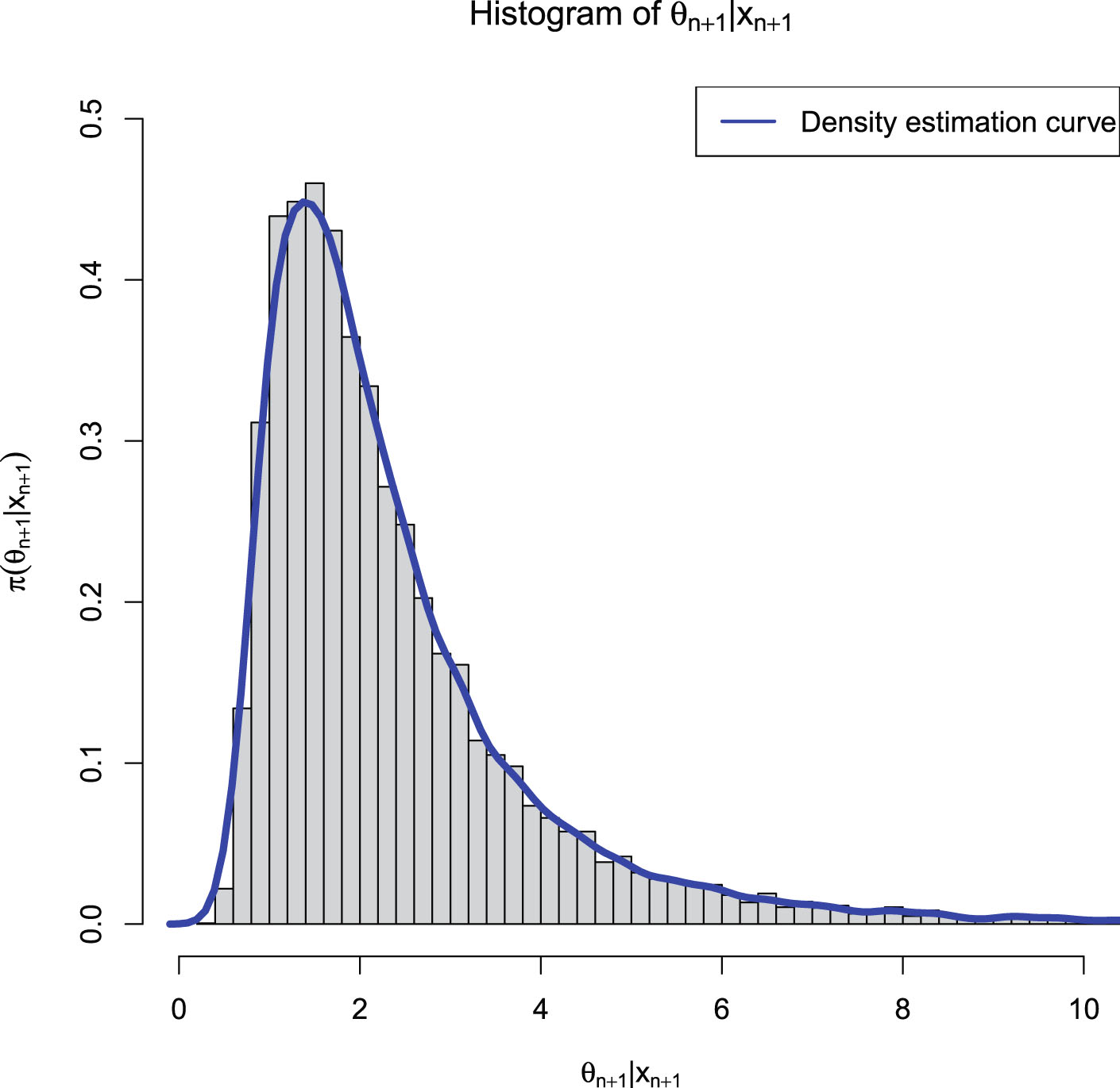
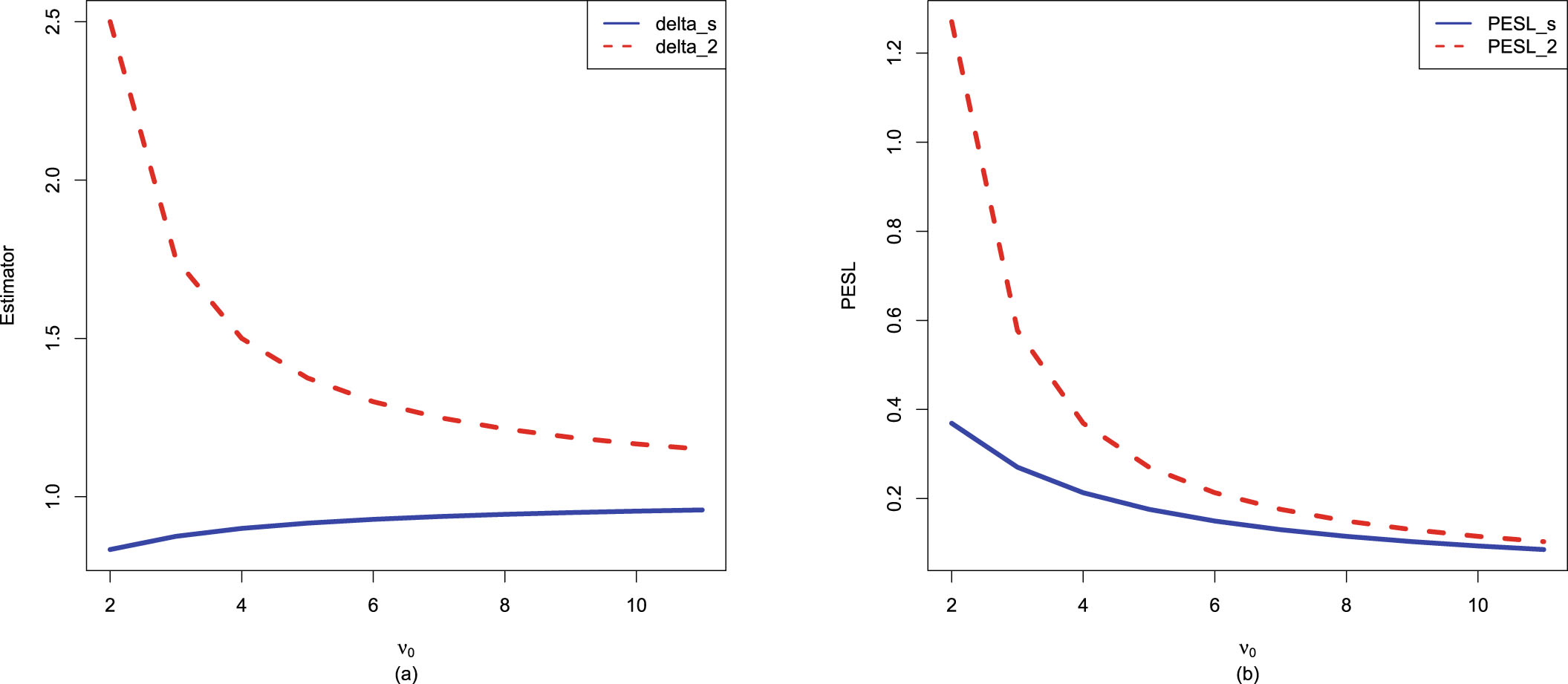
. We see from the left plot of the figure that the Bayes estimators depend on , and (6.9) is exemplified. Moreover, is an increasing function of , while is a decreasing function of . The right plot of the figure exhibits that the PESLs also depend on , and (6.10) is exemplified. Furthermore, the PESLs are decreasing functions of . In addition, table 6.1 displays the numerical values of the Bayes estimators and the PESLs in figure 6.2. In summary, the results of figure 6.2 and table 6.1 exemplify the two inequalities (6.9) and (6.10).
FIG. 6.1 — N-NIG: The histogram of  and the density estimation curve of
  .
.
and the density estimation curve of .
FIG. 6.2 — N-NIG: The Bayes estimators and the PESLs as functions of  . (a) Bayes estimators vs.
  . (b) PESLs vs.
  .
.
. (a) Bayes estimators vs. . (b) PESLs vs. .
TAB. 6.1 — N-NIG: The numerical values of the Bayes estimators and the PESLs in figure 6.2:  changes.
changes.
 |
2 | 3 | 4 | 5 | 6 | 7 | 8 | 9 | 10 | 11 |
 |
0.8333 | 0.8750 | 0.9000 | 0.9167 | 0.9286 | 0.9375 | 0.9444 | 0.9500 | 0.9545 | 0.9583 |
 |
2.5000 | 1.7500 | 1.5000 | 1.3750 | 1.3000 | 1.2500 | 1.2143 | 1.1875 | 1.1667 | 1.1500 |
 |
0.3690 | 0.2704 | 0.2131 | 0.1758 | 0.1496 | 0.1302 | 0.1152 | 0.1033 | 0.0937 | 0.0856 |
 |
1.2704 | 0.5772 | 0.3690 | 0.2704 | 0.2131 | 0.1758 | 0.1496 | 0.1302 | 0.1152 | 0.1033 |
Figure 6.3 shows the Bayes estimators and the PESLs as functions of  ,
,  ,
,  , and
, and  . We see from the left plots of the figure that the Bayes estimators depend on
  ,
,  ,
,  , and
, and  , and (6.9) is exemplified. Moreover, the Bayes estimators are first decreasing and then increasing functions of
  and
and  , and they are increasing functions of
  and
and  . The right plots of the figure exhibit that the PESLs do not depend on
  ,
,  ,
,  , and
, and  , and (6.10) is exemplified. Furthermore, tables 6.2–6.5 display the numerical values of the Bayes estimators and the PESLs in Figure 6.3. In summary, the results of figure 6.3 and tables 6.2–6.5 exemplify the two inequalities (6.9) and (6.10).
, , , and . We see from the left plots of the figure that the Bayes estimators depend on , , , and , and (6.9) is exemplified. Moreover, the Bayes estimators are first decreasing and then increasing functions of and , and they are increasing functions of and . The right plots of the figure exhibit that the PESLs do not depend on , , , and , and (6.10) is exemplified. Furthermore, tables 6.2–6.5 display the numerical values of the Bayes estimators and the PESLs in Figure 6.3. In summary, the results of figure 6.3 and tables 6.2–6.5 exemplify the two inequalities (6.9) and (6.10).
TAB. 6.2 — N-NIG: The numerical values of the Bayes estimators and the PESLs in figure 6.3:  changes.
changes.
 |
 |
 |
 |
 |
 |
0 | 1 | 2 | 3 | 4 | 5 |
 |
6.6429 | 5.4286 | 4.3571 | 3.4286 | 2.6429 | 2.0000 | 1.5000 | 1.1429 | 0.9286 | 0.8571 | 0.9286 |
 |
9.3000 | 7.6000 | 6.1000 | 4.8000 | 3.7000 | 2.8000 | 2.1000 | 1.6000 | 1.3000 | 1.2000 | 1.3000 |
 |
0.1496 | 0.1496 | 0.1496 | 0.1496 | 0.1496 | 0.1496 | 0.1496 | 0.1496 | 0.1496 | 0.1496 | 0.1496 |
 |
0.2131 | 0.2131 | 0.2131 | 0.2131 | 0.2131 | 0.2131 | 0.2131 | 0.2131 | 0.2131 | 0.2131 | 0.2131 |
In brief, the results of figures 6.2 and 6.3 exemplify that the PESLs depend only on  , but not on
  ,
,  ,
,  , and
, and  .
.
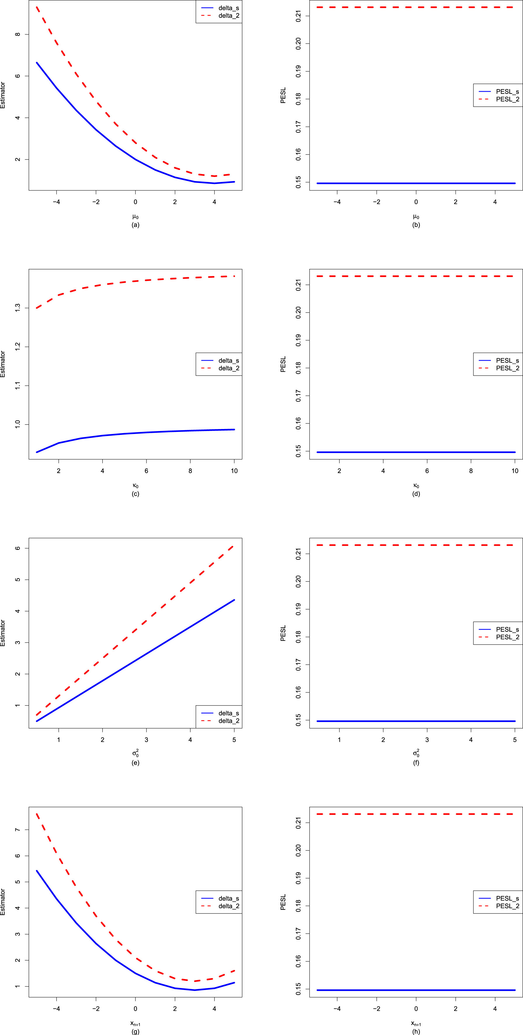
, but not on , , , and .
FIG. 6.3 — N-NIG: The Bayes estimators and the PESLs as functions of  ,
,  ,
,  , and
, and  . (a), (c), (e), (g) Bayes estimators vs.
  ,
,  ,
,  , and
, and  . (b), (d), (f), (h) PESLs vs.
  ,
,  ,
,  , and
, and  .
.
, , , and . (a), (c), (e), (g) Bayes estimators vs. , , , and . (b), (d), (f), (h) PESLs vs. , , , and .
TAB. 6.3 — N-NIG: The numerical values of the Bayes estimators and the PESLs in figure 6.3:  changes.
changes.
 |
1 | 2 | 3 | 4 | 5 | 6 | 7 | 8 | 9 | 10 |
 |
0.9286 | 0.9524 | 0.9643 | 0.9714 | 0.9762 | 0.9796 | 0.9821 | 0.9841 | 0.9857 | 0.9870 |
 |
1.3000 | 1.3333 | 1.3500 | 1.3600 | 1.3667 | 1.3714 | 1.3750 | 1.3778 | 1.3800 | 1.3818 |
 |
0.1496 | 0.1496 | 0.1496 | 0.1496 | 0.1496 | 0.1496 | 0.1496 | 0.1496 | 0.1496 | 0.1496 |
 |
0.2131 | 0.2131 | 0.2131 | 0.2131 | 0.2131 | 0.2131 | 0.2131 | 0.2131 | 0.2131 | 0.2131 |
TAB. 6.4 — N-NIG: The numerical values of the Bayes estimators and the PESLs in figure 6.3:  changes.
changes.
 |
0.5 | 1 | 1.5 | 2 | 2.5 | 3 | 3.5 | 4 | 4.5 | 5 |
 |
0.5000 | 0.9286 | 1.3571 | 1.7857 | 2.2143 | 2.6429 | 3.0714 | 3.5000 | 3.9286 | 4.3571 |
 |
0.7000 | 1.3000 | 1.9000 | 2.5000 | 3.1000 | 3.7000 | 4.3000 | 4.9000 | 5.5000 | 6.1000 |
 |
0.1496 | 0.1496 | 0.1496 | 0.1496 | 0.1496 | 0.1496 | 0.1496 | 0.1496 | 0.1496 | 0.1496 |
 |
0.2131 | 0.2131 | 0.2131 | 0.2131 | 0.2131 | 0.2131 | 0.2131 | 0.2131 | 0.2131 | 0.2131 |
TAB. 6.5 — N-NIG: The numerical values of the Bayes estimators and the PESLs in figure 6.3:  changes.
changes.
 |
 |
 |
 |
 |
 |
0 | 1 | 2 | 3 | 4 | 5 |
 |
5.4286 | 4.3571 | 3.4286 | 2.6429 | 2.0000 | 1.5000 | 1.1429 | 0.9286 | 0.8571 | 0.9286 | 1.1429 |
 |
7.6000 | 6.1000 | 4.8000 | 3.7000 | 2.8000 | 2.1000 | 1.6000 | 1.3000 | 1.2000 | 1.3000 | 1.6000 |
 |
0.1496 | 0.1496 | 0.1496 | 0.1496 | 0.1496 | 0.1496 | 0.1496 | 0.1496 | 0.1496 | 0.1496 | 0.1496 |
 |
0.2131 | 0.2131 | 0.2131 | 0.2131 | 0.2131 | 0.2131 | 0.2131 | 0.2131 | 0.2131 | 0.2131 | 0.2131 |
Since the Bayes estimators  and
and  and the PESLs
  and
and  depend on
  and
and  , where
  and
and  , we can plot the surfaces of the Bayes estimators and the PESLs on the domain
  via the R function persp3d() in the R package rgl (see Zhang et al. (2017, 2019b); Sun et al. (2021); Adler et al. (2017)). We remark that the R function persp() in the R package graphics can not add another surface to the existing surface, but persp3d() can. Moreover, persp3d() allows one to rotate the perspective plots of the surface according to one’s wishes. Figure 6.4 plots the surfaces of the Bayes estimators and the PESLs, and the surfaces of the differences of the Bayes estimators and the PESLs. The domain for
  is
is  for all the plots. a is for
  and b is for
  in the axes of all the plots. The red surface is for
  and the blue surface is for
  in the upper two plots. From the left two plots of the figure, we see that
  for all
  on
on  , which exemplifies (6.9). From the right two plots of the figure, we see that
  for all
  on
on  , which exemplifies (6.10). The results of the figure exemplify the theoretical studies of (6.9) and (6.10).
and and the PESLs and depend on and , where and , we can plot the surfaces of the Bayes estimators and the PESLs on the domain via the R function persp3d() in the R package rgl (see Zhang et al. (2017, 2019b); Sun et al. (2021); Adler et al. (2017)). We remark that the R function persp() in the R package graphics can not add another surface to the existing surface, but persp3d() can. Moreover, persp3d() allows one to rotate the perspective plots of the surface according to one’s wishes. Figure 6.4 plots the surfaces of the Bayes estimators and the PESLs, and the surfaces of the differences of the Bayes estimators and the PESLs. The domain for is for all the plots. a is for and b is for in the axes of all the plots. The red surface is for and the blue surface is for in the upper two plots. From the left two plots of the figure, we see that for all on , which exemplifies (6.9). From the right two plots of the figure, we see that for all on , which exemplifies (6.10). The results of the figure exemplify the theoretical studies of (6.9) and (6.10).
6.3.2 Consistencies of the Moment Estimators and the MLEs
In this subsection, similar to subsection 1.8.1, we will numerically exemplify that the moment estimators  and the MLEs
  are consistent estimators of the hyperparameters
  of the hierarchical normal and normal-inverse-gamma model (6.2). The motivation of this subsection is that in Theorems 6.2 and 6.3, we have theoretically shown that the moment estimators and the MLEs are consistent estimators of the hyperparameters. Note that only
  are used in this subsection.
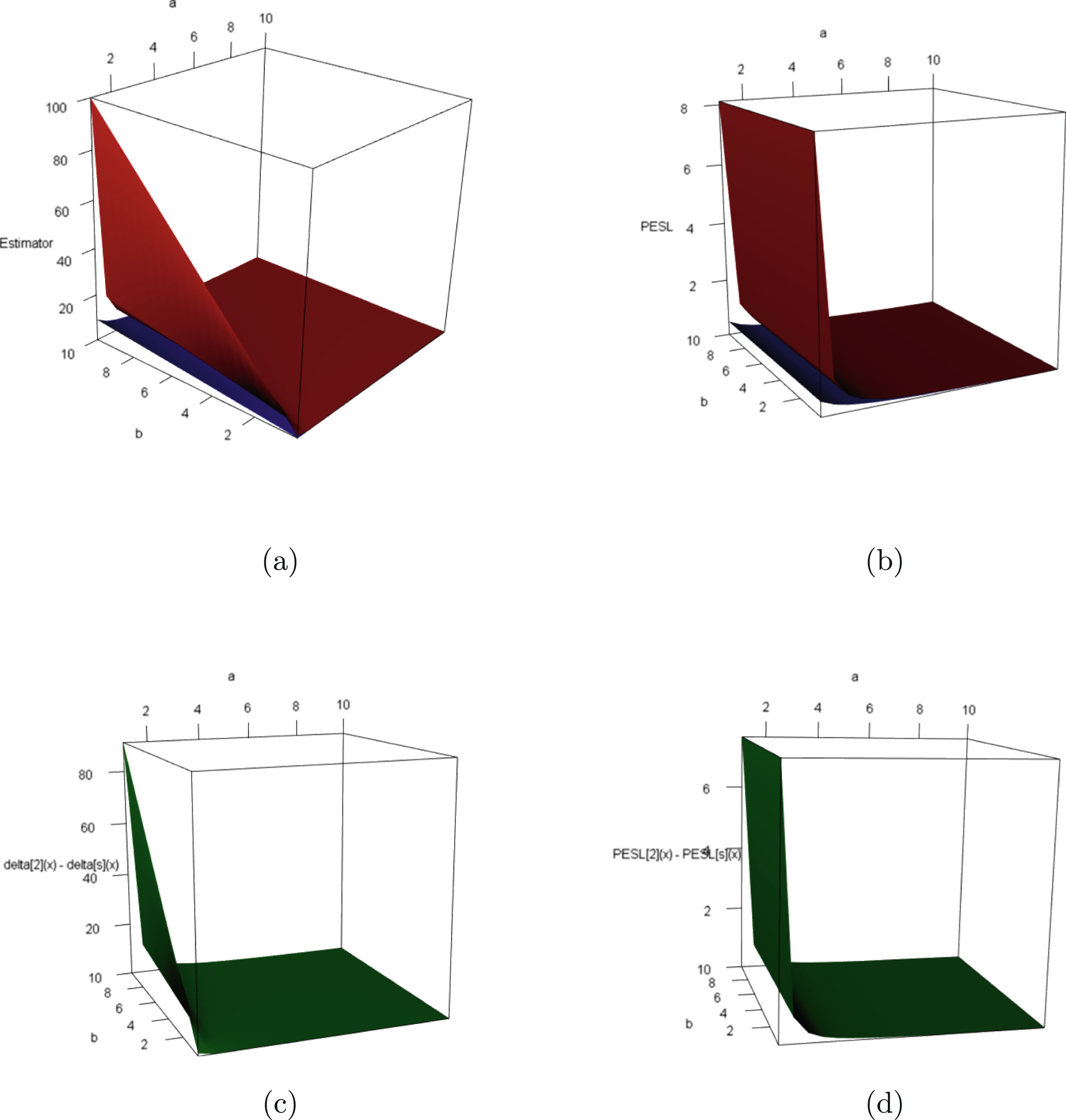
and the MLEs are consistent estimators of the hyperparameters of the hierarchical normal and normal-inverse-gamma model (6.2). The motivation of this subsection is that in Theorems 6.2 and 6.3, we have theoretically shown that the moment estimators and the MLEs are consistent estimators of the hyperparameters. Note that only are used in this subsection.
FIG. 6.4 — N-NIG: (a) The Bayes estimators as functions of  and
and  . (b) The PESLs as functions of
  and
and  . (c) The surface of
  which is positive for all
  on
on  . (d) The surface of
  which is also positive for all
  on
on  .
.
and . (b) The PESLs as functions of and . (c) The surface of which is positive for all on . (d) The surface of which is also positive for all on .
First, we will numerically exemplify that the sample  generated from the model (6.1) can not be used to estimate the hyperparameters
  , while the sample
  generated from the model (6.2) can be used to estimate the hyperparameters
  , where
  . Moreover, we will exemplify that the moment estimators and the MLEs of
  can correctly estimate the true hyperparameter
  regardless of the
  and
and  values.
generated from the model (6.1) can not be used to estimate the hyperparameters , while the sample generated from the model (6.2) can be used to estimate the hyperparameters , where . Moreover, we will exemplify that the moment estimators and the MLEs of can correctly estimate the true hyperparameter regardless of the and values.
The histograms of the samples and their density curves are plotted in figure 6.5. From the figure, we observe the following facts.
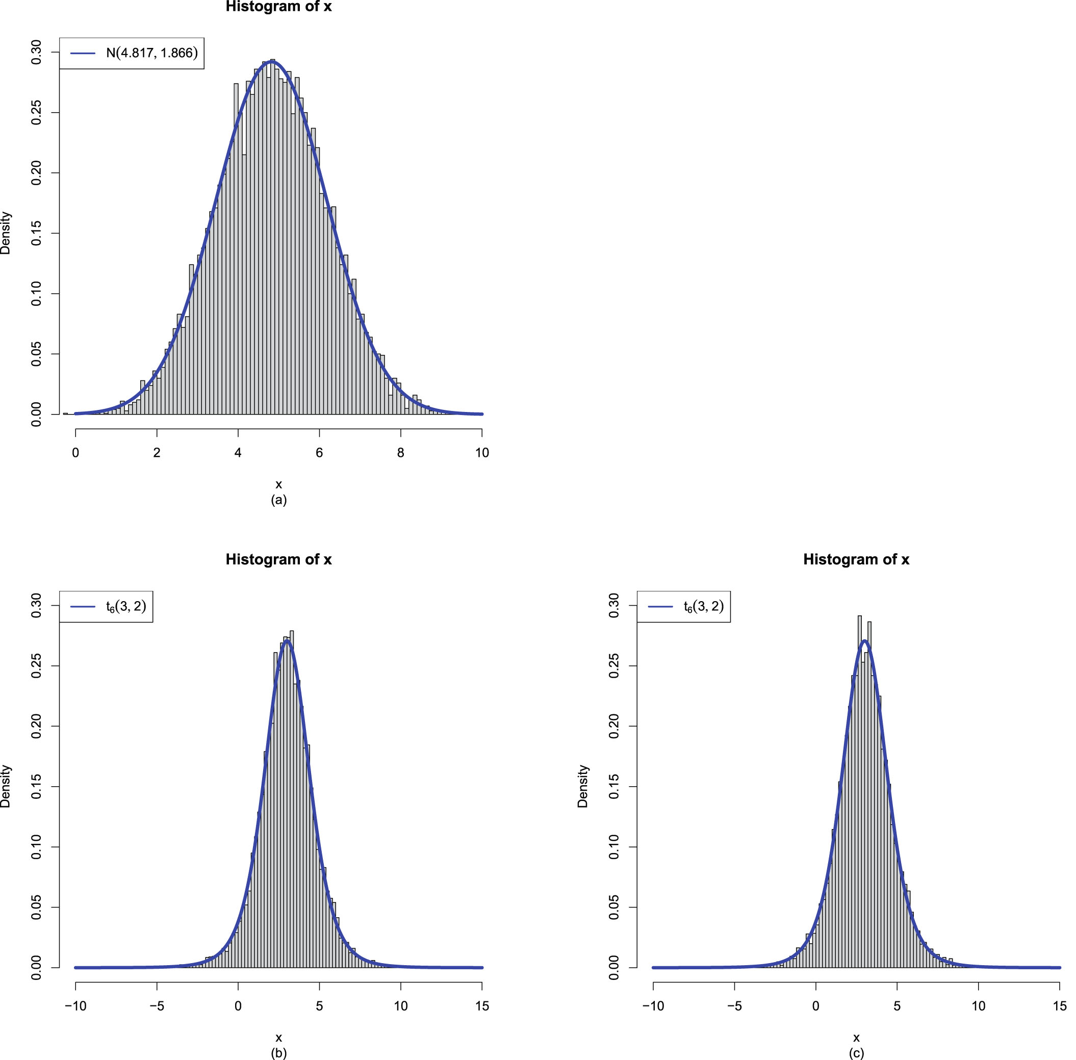
FIG. 6.5 — N-NIG: The histograms of the samples and their density curves. (a)  generated from the model (6.1) with
  and
and  . (b)
. (b)  generated from the model (6.2) with
  and
and  . (c)
. (c)  generated from the model (6.2) with
  and
and  .
.
generated from the model (6.1) with and . (b) generated from the model (6.2) with and . (c) generated from the model (6.2) with and .
1. Plot (a): The sample  generated from the model (6.1) are iid from
  with
with  and
and  .
.
generated from the model (6.1) are iid from with and .
2. Plots (b) and (c): The sample  are generated from the model (6.2) with
  and
and  . The sample
  are generated from the model (6.2) with
  and
and  . Although
  and
and  are different in the two plots,
  is the same. Therefore, the two samples
  and
and  are from the same marginal distribution
  with
with  .
.
are generated from the model (6.2) with and . The sample are generated from the model (6.2) with and . Although and are different in the two plots, is the same. Therefore, the two samples and are from the same marginal distribution with .
The moment estimators and the MLEs of the hyperparameters  for the samples
  ,
,  , and
, and  are summarized in table 6.6. From the table, we observe the following facts.
for the samples , , and are summarized in table 6.6. From the table, we observe the following facts.
1. The moment estimators of the hyperparameters  for sample
  are far away from the true hyperparameters
  , and thus the samples generated from the model (6.1) can not be used to estimate the hyperparameters
  .
.
for sample are far away from the true hyperparameters , and thus the samples generated from the model (6.1) can not be used to estimate the hyperparameters .
2. For  , since the moment estimator of
  is
is  which is negative, the MLE method fails to iterate, and thus the MLEs of the hyperparameters
  are equal to the moment estimators.
, since the moment estimator of is which is negative, the MLE method fails to iterate, and thus the MLEs of the hyperparameters are equal to the moment estimators.
3. For  and
and  , the moment estimators and the MLEs of the hyperparameters
  are close to the true hyperparameters
  , and thus the samples generated from the model (6.2) can be used to estimate the hyperparameters
  .
.
and , the moment estimators and the MLEs of the hyperparameters are close to the true hyperparameters , and thus the samples generated from the model (6.2) can be used to estimate the hyperparameters .
4. The sample  is generated from the model (6.2) with
  , while the sample
  is generated from the model (6.2) with
  . Although
  and
and  are different for the two samples
  and
and  ,
,  is the same. We find that both the moment method and the MLE method correctly estimate the true hyperparameter
  for the two samples
  and
and  .
.
is generated from the model (6.2) with , while the sample is generated from the model (6.2) with . Although and are different for the two samples and , is the same. We find that both the moment method and the MLE method correctly estimate the true hyperparameter for the two samples and .
5. For  and
and  , the MLEs are closer to the true hyperparameters
  than the moment estimators for this simulation.
and , the MLEs are closer to the true hyperparameters than the moment estimators for this simulation.
TAB. 6.6 — N-NIG: The moment estimators and the MLEs of the hyperparameters  for the samples
  ,
,  , and
, and  .
.
for the samples , , and .
| Moment estimators | MLEs | |
 |
 |
 |
 |
 |
 |
 |
 |
 |
Now, let us exemplify that the moment estimators  and the MLEs
  are consistent estimators of the hyperparameters
  . The frequencies of the moment estimators and the MLEs of the hyperparameters as
  varies for
  and
and  , 0.5, and 0.1 are reported in table 6.7. Note that the data in this simulation are simulated according to the hierarchical normal and normal-inverse-gamma model (6.2) with
  and
and  . Other numerical values of the hyperparameters can also be specified. From the table, we observe the following facts.
and the MLEs are consistent estimators of the hyperparameters . The frequencies of the moment estimators and the MLEs of the hyperparameters as varies for and , 0.5, and 0.1 are reported in table 6.7. Note that the data in this simulation are simulated according to the hierarchical normal and normal-inverse-gamma model (6.2) with and . Other numerical values of the hyperparameters can also be specified. From the table, we observe the following facts.
1. Given  , 0.5, or 0.1, the frequencies of the estimators tend to 0 as
  increases to infinity, which means that the moment estimators and the MLEs are consistent estimators of the hyperparameters. For
  , the frequencies of the estimators
  and
and  are still very large (
 for all the cases). However, we observe the tendencies of declining to 0 as
  increases to infinity.
, 0.5, or 0.1, the frequencies of the estimators tend to 0 as increases to infinity, which means that the moment estimators and the MLEs are consistent estimators of the hyperparameters. For , the frequencies of the estimators and are still very large ( for all the cases). However, we observe the tendencies of declining to 0 as increases to infinity.
2. Comparing the frequencies corresponding to  , 0.5, and 0.1, we observe that as
  gets smaller, the frequencies tend to be larger, since the constraints

, 0.5, and 0.1, we observe that as gets smaller, the frequencies tend to be larger, since the constraints
are easier to meet.
3. Comparing the moment estimators and the MLEs of the hyperparameters  ,
,  , and
, and  , we see that the frequencies of the MLEs are smaller than those of the moment estimators for large
  , which means that the MLEs are better than the moment estimators when estimating the hyperparameters in terms of consistency.
, , and , we see that the frequencies of the MLEs are smaller than those of the moment estimators for large , which means that the MLEs are better than the moment estimators when estimating the hyperparameters in terms of consistency.
6.3.3 Goodness-of-Fit of the Model: KS Test
In this subsection, similar to subsection 1.8.2, we will calculate the goodness-of-fit of the hierarchical normal and normal-inverse-gamma model (6.2) to the simulated data. The motivation of this subsection is that we want to check whether the marginal distribution of the hierarchical normal and normal-inverse-gamma model (6.2) fits the simulated data well. Note that only  are used in this subsection.
are used in this subsection.
TAB. 6.7 — N-NIG: The frequencies of the moment estimators and the MLEs of the hyperparameters as  varies for
  and
and  , 0.5, and 0.1.
varies for and , 0.5, and 0.1.
| Moment estimators | MLEs | ||||||
 |
 |
 |
 |
 |
 |
 |
|
 |
1e4 | 0.00 | 0.24 | 0.00 | 0.00 | 0.03 | 0.00 |
| 2e4 | 0.00 | 0.23 | 0.00 | 0.00 | 0.00 | 0.00 | |
| 4e4 | 0.00 | 0.06 | 0.00 | 0.00 | 0.00 | 0.00 | |
| 8e4 | 0.00 | 0.01 | 0.00 | 0.00 | 0.00 | 0.00 | |
| 16e4 | 0.00 | 0.00 | 0.00 | 0.00 | 0.00 | 0.00 | |
 |
1e4 | 0.00 | 0.48 | 0.00 | 0.00 | 0.16 | 0.00 |
| 2e4 | 0.00 | 0.40 | 0.00 | 0.00 | 0.04 | 0.00 | |
| 4e4 | 0.00 | 0.33 | 0.00 | 0.00 | 0.00 | 0.00 | |
| 8e4 | 0.00 | 0.19 | 0.00 | 0.00 | 0.00 | 0.00 | |
| 16e4 | 0.00 | 0.10 | 0.00 | 0.00 | 0.00 | 0.00 | |
 |
1e4 | 0.00 | 0.81 | 0.36 | 0.00 | 0.84 | 0.03 |
| 2e4 | 0.00 | 0.87 | 0.34 | 0.00 | 0.62 | 0.00 | |
| 4e4 | 0.00 | 0.82 | 0.21 | 0.00 | 0.52 | 0.00 | |
| 8e4 | 0.00 | 0.81 | 0.10 | 0.00 | 0.43 | 0.00 | |
| 16e4 | 0.00 | 0.70 | 0.04 | 0.00 | 0.27 | 0.00 | |
In our problem, the null hypothesis specifies that
 where
where  is the marginal distribution of the hierarchical normal and normal-inverse-gamma model (6.2). The marginal density of the
  distribution is given by (6.12), which is obviously one-dimensional and continuous. Hence, the KS test can be utilized as a measure of the goodness-of-fit.
is the marginal distribution of the hierarchical normal and normal-inverse-gamma model (6.2). The marginal density of the distribution is given by (6.12), which is obviously one-dimensional and continuous. Hence, the KS test can be utilized as a measure of the goodness-of-fit.
Note that the data in this subsection are simulated according to the hierarchical normal and normal-inverse-gamma model (6.2) with  and
and  . Other numerical values of the hyperparameters can also be specified.
and . Other numerical values of the hyperparameters can also be specified.
The results of the KS test goodness-of-fit of the model (6.2) to the simulated data are reported in table 6.8. In the table, the hyperparameters  ,
,  , and
, and  are estimated by three methods. The first method is the oracle method, in that we know the hyperparameters
  ,
,  , and
, and  . The second method is the moment method, in which the hyperparameters are estimated by their moment estimators (see Theorem 6.2). The third method is the MLE method, in which the hyperparameters are estimated by their MLEs (see Theorem 6.3). In the table, the sample size is
  , and the number of simulations is
  .
.
, , and are estimated by three methods. The first method is the oracle method, in that we know the hyperparameters , , and . The second method is the moment method, in which the hyperparameters are estimated by their moment estimators (see Theorem 6.2). The third method is the MLE method, in which the hyperparameters are estimated by their MLEs (see Theorem 6.3). In the table, the sample size is , and the number of simulations is .
From table 6.8, we observe the following facts.
1. The  values for the three methods are respectively given by 0.0268, 0.0239, and 0.0204, which means that the MLE method is the best method, the moment method is the second-best method, and the oracle method is the worst method. A possible explanation for this phenomenon is that in (1.23), the empirical cdf
  is based on data, and the population cdfs
  for the MLE method and the moment method are also based on data, while the population cdf
  for the oracle method is not based on data.
values for the three methods are respectively given by 0.0268, 0.0239, and 0.0204, which means that the MLE method is the best method, the moment method is the second-best method, and the oracle method is the worst method. A possible explanation for this phenomenon is that in (1.23), the empirical cdf is based on data, and the population cdfs for the MLE method and the moment method are also based on data, while the population cdf for the oracle method is not based on data.
2. The  values for the three methods are respectively given by 0.5230, 0.6245, and 0.7674, which also means that the MLE method ranks first, the moment method ranks second, and the oracle method ranks third. The possible explanation for this phenomenon is described in the previous paragraph.
values for the three methods are respectively given by 0.5230, 0.6245, and 0.7674, which also means that the MLE method ranks first, the moment method ranks second, and the oracle method ranks third. The possible explanation for this phenomenon is described in the previous paragraph.
3. The  values for the three methods are respectively given by 0.20, 0.16, and 0.64. The
  value for the MLE method accounts for over half of the
  simulations. The order of preference for the three methods is the MLE method, the oracle method, and the moment method.
values for the three methods are respectively given by 0.20, 0.16, and 0.64. The value for the MLE method accounts for over half of the simulations. The order of preference for the three methods is the MLE method, the oracle method, and the moment method.
4. The  values for the three methods are respectively given by 0.20, 0.16, and 0.64. A small
  value corresponds to a large p-value. Hence, the smallest
  value corresponds to the largest p-value. Therefore, the
  value and the
  value for the three methods are the same. The order of preference for the three methods is the MLE method, the oracle method, and the moment method.
values for the three methods are respectively given by 0.20, 0.16, and 0.64. A small value corresponds to a large p-value. Hence, the smallest value corresponds to the largest p-value. Therefore, the value and the value for the three methods are the same. The order of preference for the three methods is the MLE method, the oracle method, and the moment method.
5. The  values for the three methods are respectively given by
  ,
,  , and
, and  . The
. The  values for the three methods are nearly
  , which means that the three methods have good performances in terms of goodness-of-fit.
values for the three methods are respectively given by , , and . The values for the three methods are nearly , which means that the three methods have good performances in terms of goodness-of-fit.
6. In summary, for the five indices ( ,
,  ,
,  ,
,  ,
,  ), the MLE method always ranks first. Comparing the moment method and the MLE method, we find that the MLE method has a better performance than the moment method in terms of all five indices.
, , , , ), the MLE method always ranks first. Comparing the moment method and the MLE method, we find that the MLE method has a better performance than the moment method in terms of all five indices.
The boxplots of the  values and the p-values for the three methods are displayed in figure 6.6. From the figure, we observe the following facts.
values and the p-values for the three methods are displayed in figure 6.6. From the figure, we observe the following facts.
TAB. 6.8 — N-NIG: The results of the KS test goodness-of-fit of the model (6.2) to the simulated data.
 |
 |
 |
|
 |
0.0268 | 0.0239 | 0.0204 |
 |
0.5230 | 0.6245 | 0.7674 |
 |
0.20 | 0.16 | 0.64 |
 |
0.20 | 0.16 | 0.64 |
 |
0.98 | 0.99 | 0.99 |
1. The  values of the oracle method are larger than those of the other two methods. Since for the
  value, the smaller the better, the order of preference for the three methods is the MLE method, the moment method, and the oracle method.
values of the oracle method are larger than those of the other two methods. Since for the value, the smaller the better, the order of preference for the three methods is the MLE method, the moment method, and the oracle method.
2. The p-values of the oracle method are smaller than those of the other two methods. Since for the p-value, the larger the better, the order of preference for the three methods is the MLE method, the moment method, and the oracle method.
3. Small  values correspond to large p-values, and large
  values correspond to small p-values.
values correspond to large p-values, and large values correspond to small p-values.
4. The MLE method has a better performance than the moment method in terms of the  values and the p-values.
values and the p-values.
6.3.4 Marginal Densities for Various Hyperparameters
In this subsection, we will plot the marginal densities of the hierarchical normal and normal-inverse-gamma model (6.2) for various hyperparameters  ,
,  ,
,  , and
, and  . The motivation of this subsection is that we want to know what kind of data can be modeled by the hierarchical normal and normal-inverse-gamma model (6.2). Note that the marginal density of
  is given by (6.6) specified by four hyperparameters
  ,
,  ,
,  , and
, and  . We will explore how the marginal densities change around the marginal density with hyperparameters specified by
  ,
,  ,
,  , and
, and  . Other numerical values of the hyperparameters can also be specified.
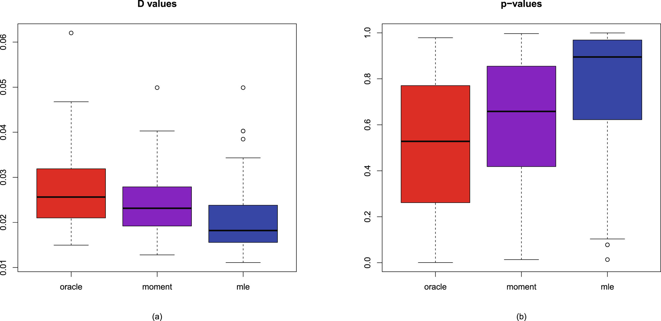
, , , and . The motivation of this subsection is that we want to know what kind of data can be modeled by the hierarchical normal and normal-inverse-gamma model (6.2). Note that the marginal density of is given by (6.6) specified by four hyperparameters , , , and . We will explore how the marginal densities change around the marginal density with hyperparameters specified by , , , and . Other numerical values of the hyperparameters can also be specified.
FIG. 6.6 — N-NIG: The boxplots of the  values and the p-values for the three methods. (a)
  values. (b) p-values.
values and the p-values for the three methods. (a) values. (b) p-values.
Figure 6.7 plots the marginal densities for varied  , holding
  ,
,  , and
, and  fixed. From the figure we see that as
  increases, the marginal density shifts to the right, while keeping the shape of the curve unchanged. That is,
  is a location parameter. Moreover, all the marginal densities are symmetric about the mean
  .
.
, holding , , and fixed. From the figure we see that as increases, the marginal density shifts to the right, while keeping the shape of the curve unchanged. That is, is a location parameter. Moreover, all the marginal densities are symmetric about the mean .
Figure 6.8 plots the marginal densities for varied  , holding
  ,
,  , and
, and  fixed. From the figure, we see that as
  increases, the peak value of the marginal density increases. In other words, the variance of the marginal density decreases as
 (6.22)
is a decreasing function of
(6.22)
is a decreasing function of  . Moreover, all the marginal densities are symmetric about the mean
  .
.
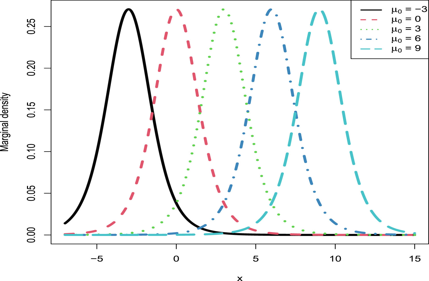
, holding , , and fixed. From the figure, we see that as increases, the peak value of the marginal density increases. In other words, the variance of the marginal density decreases as
(6.22)
. Moreover, all the marginal densities are symmetric about the mean .
FIG. 6.7 — N-NIG: The marginal densities for varied  , holding
  ,
,  , and
, and  fixed.
, holding , , and fixed.
Figure 6.9 plots the marginal densities for varied  , holding
  ,
,  , and
, and  fixed. From the figure, we see that as
  increases, the peak value of the marginal density increases. In other words, the variance of the marginal density decreases, as (6.22) is a decreasing function of
  . Moreover, all the marginal densities are symmetric about the mean
  .
.
, holding , , and fixed. From the figure, we see that as increases, the peak value of the marginal density increases. In other words, the variance of the marginal density decreases, as (6.22) is a decreasing function of . Moreover, all the marginal densities are symmetric about the mean .
Figure 6.10 plots the marginal densities for varied  , holding
  ,
,  , and
, and  fixed. From the figure, we see that as
  increases, the peak value of the marginal density decreases. In other words, the variance of the marginal density increases, as (6.22) is an increasing function of
  . Moreover, all the marginal densities are symmetric about the mean
  .
.
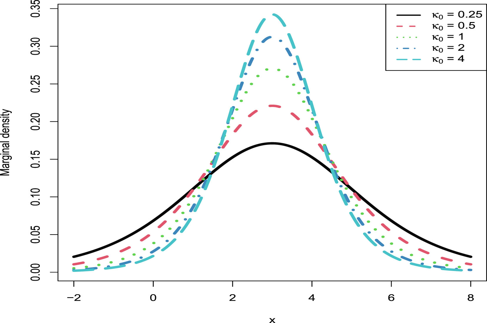
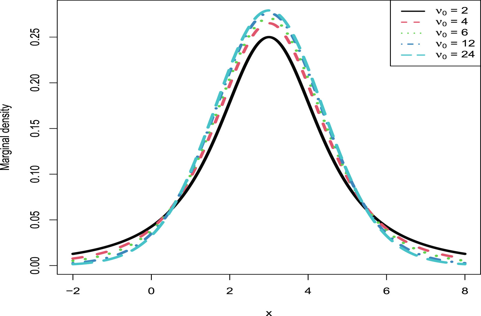
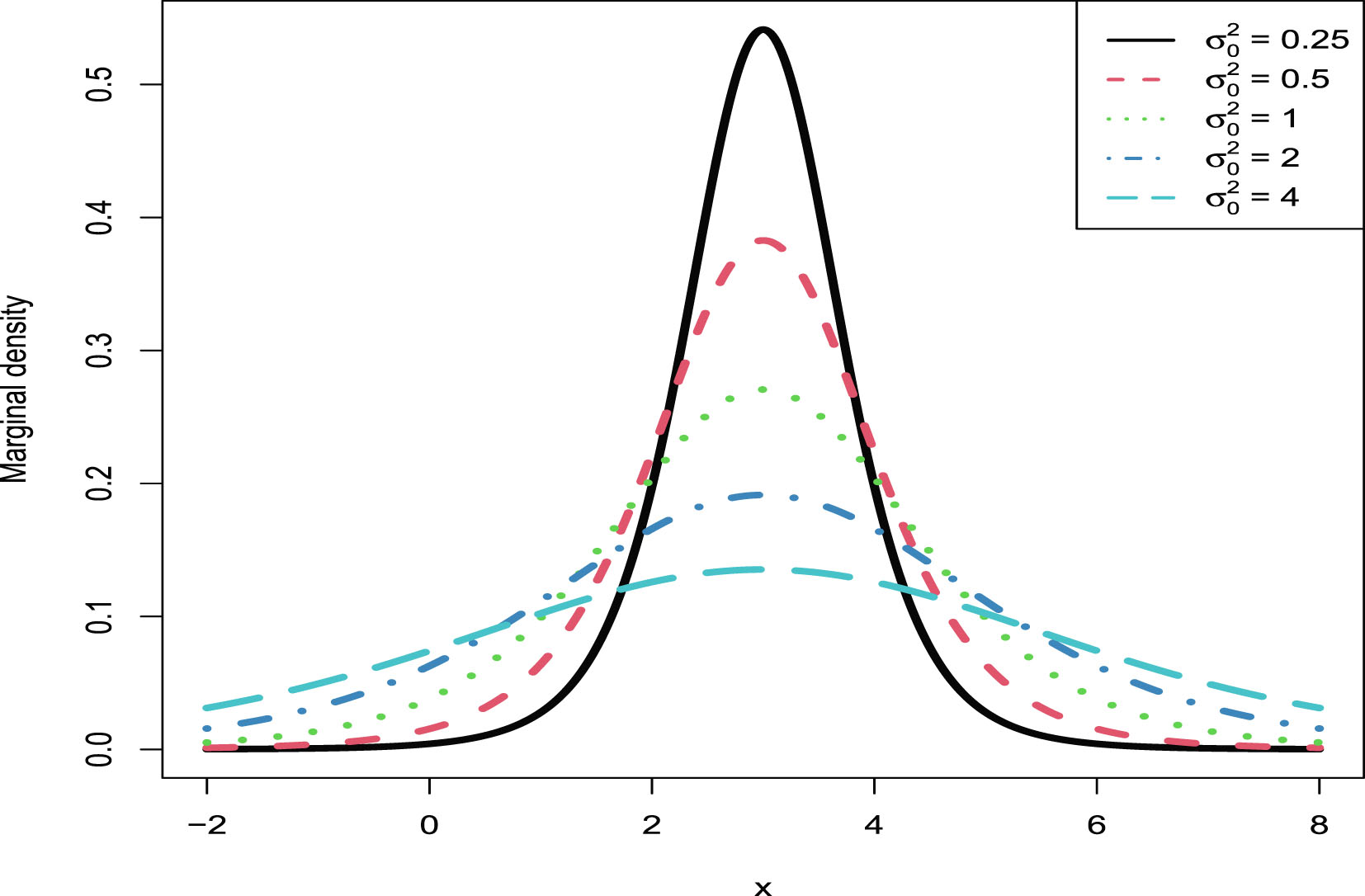
, holding , , and fixed. From the figure, we see that as increases, the peak value of the marginal density decreases. In other words, the variance of the marginal density increases, as (6.22) is an increasing function of . Moreover, all the marginal densities are symmetric about the mean .
FIG. 6.8 — N-NIG: The marginal densities for varied  , holding
  ,
,  , and
, and  fixed.
, holding , , and fixed.
FIG. 6.9 — N-NIG: The marginal densities for varied  , holding
  ,
,  , and
, and  fixed.
, holding , , and fixed.
FIG. 6.10 — N-NIG: The marginal densities for varied  , holding
  ,
,  , and
, and  fixed.
, holding , , and fixed.
6.4 A Real Data Example
In this section, we exploit the poverty level data. The data represent percentages of all persons below the poverty level. The sample is from a random collection of  cities in the Western U.S. Source: County and City Data Book, 12th edition, U.S. Department of Commerce.
cities in the Western U.S. Source: County and City Data Book, 12th edition, U.S. Department of Commerce.
The histogram of the sample  and its density estimation curve is depicted in figure 6.11. From the figure, we see that the data are roughly symmetric about 0.15.
and its density estimation curve is depicted in figure 6.11. From the figure, we see that the data are roughly symmetric about 0.15.
The estimators of the hyperparameters  ,
,  , and
, and  , the goodness-of-fit of the model, the empirical Bayes estimators of the variance parameter of the normal distribution with a conjugate normal-inverse-gamma prior and the PESLs, and the mean and variance of the poverty level data by the moment method and the MLE method are summarized in table 6.9. From the table, we observe the following facts.
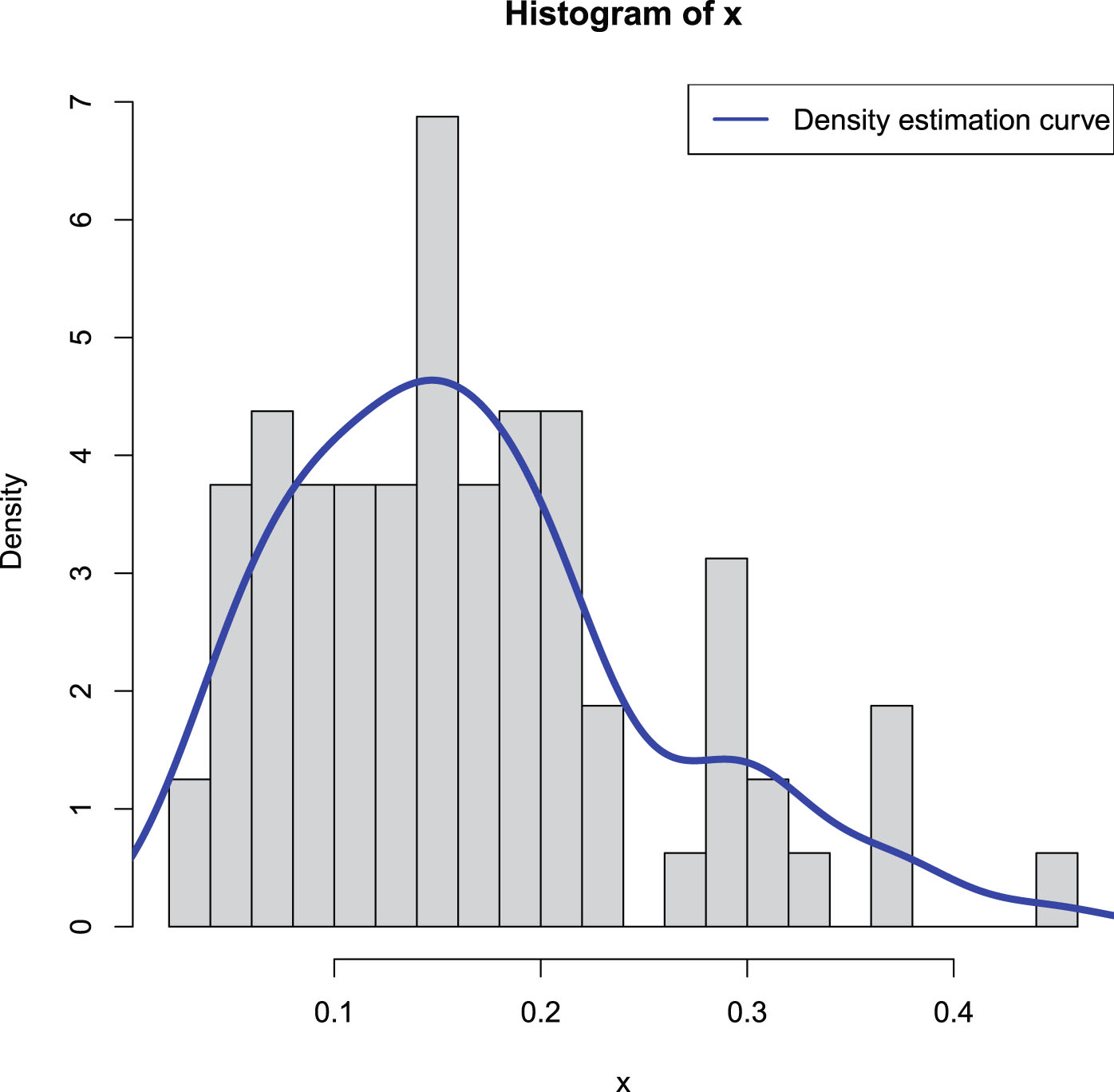
, , and , the goodness-of-fit of the model, the empirical Bayes estimators of the variance parameter of the normal distribution with a conjugate normal-inverse-gamma prior and the PESLs, and the mean and variance of the poverty level data by the moment method and the MLE method are summarized in table 6.9. From the table, we observe the following facts.
FIG. 6.11 — N-NIG: The histogram of the sample  and its density estimation curve.
and its density estimation curve.
1. The moment estimator of the hyperparameter  is equal to the sample mean
  of the first
  observations. It is interesting to note that the MLE of the hyperparameter
  is equal to 0.1619865, which is very similar to the moment estimator of the hyperparameter
  . Moreover, the moment estimator and the MLE of the hyperparameter
  are also very similar, and they are close to 0.006. But the moment estimator and the MLE of the hyperparameter
  are quite different. This does not mean that the hierarchical normal and normal-inverse-gamma model (6.2) does not fit the real data, nor mean that the moment estimator and the MLE are not consistent estimators of the hyperparameter
  . The reason for the big difference between the two estimators is that the sample size
  is too small. Of course, the MLE of the hyperparameter
  is more reliable, as assured from the previous figures and tables in the simulations section.
is equal to the sample mean of the first observations. It is interesting to note that the MLE of the hyperparameter is equal to 0.1619865, which is very similar to the moment estimator of the hyperparameter . Moreover, the moment estimator and the MLE of the hyperparameter are also very similar, and they are close to 0.006. But the moment estimator and the MLE of the hyperparameter are quite different. This does not mean that the hierarchical normal and normal-inverse-gamma model (6.2) does not fit the real data, nor mean that the moment estimator and the MLE are not consistent estimators of the hyperparameter . The reason for the big difference between the two estimators is that the sample size is too small. Of course, the MLE of the hyperparameter is more reliable, as assured from the previous figures and tables in the simulations section.
2. We use the KS test as a measure of the goodness-of-fit. The p-value of the moment method is  , and thus the
  distribution with
  ,
,  , and
, and  estimated by their moment estimators fits the sample
  well. Moreover, the p-value of the MLE method is
  , and thus the
  distribution with
  ,
,  , and
, and  estimated by their MLEs fits the sample
  even better. When comparing the two methods, we observe that the
  value of the MLEs is smaller, and the p-value of the MLEs is larger, which means that the
  distribution with the hyperparameters
  ,
,  , and
, and  estimated by the MLEs has a better fit to the sample
  than that estimated by the moment estimators.
, and thus the distribution with , , and estimated by their moment estimators fits the sample well. Moreover, the p-value of the MLE method is , and thus the distribution with , , and estimated by their MLEs fits the sample even better. When comparing the two methods, we observe that the value of the MLEs is smaller, and the p-value of the MLEs is larger, which means that the distribution with the hyperparameters , , and estimated by the MLEs has a better fit to the sample than that estimated by the moment estimators.
3. When the hyperparameters are estimated by the MLE method, we see that

and

When the hyperparameters are estimated by the moment method, we observe a similar phenomenon for the Bayes estimators and the PESLs. Consequently, the two inequalities (6.9) and (6.10) are exemplified.
4. The mean of  (the poverty level data) is estimated by
  . By (6.22), the variance of
  is estimated by
  . It is interesting to note that the mean and variance of
  by the two methods are very similar, although the estimators of the hyperparameters are quite different. Moreover, it is worthy to mention that


(the poverty level data) is estimated by . By (6.22), the variance of is estimated by . It is interesting to note that the mean and variance of by the two methods are very similar, although the estimators of the hyperparameters are quite different. Moreover, it is worthy to mention that
for the MLE method. The mean and variance of  are similar for the moment method. Therefore, the variance of
  is quite small, not large!
are similar for the moment method. Therefore, the variance of is quite small, not large!
TAB. 6.9 — N-NIG: The estimators of the hyperparameters, the goodness-of-fit of the model, the empirical Bayes estimators of the variance parameter of the normal distribution and the PESLs, and the mean and variance of the poverty level data by the moment method and the MLE method.
| Moment method | MLE method | ||
| Estimators of the hyperparameters |  |
 |
 |
 |
 |
 |
|
 |
 |
 |
|
| Goodness-of-fit of the model |  |
0.0909 | 0.0708 |
| p-value | 0.5313 | 0.8233 | |
| Empirical Bayes estimators and PESLs |  |
0.0023464 | 0.0032576 |
 |
0.0035396 | 0.0038348 | |
 |
0.1779193 | 0.0771456 | |
 |
0.2753140 | 0.0912061 | |
| Mean and variance of the poverty level data |  |
0.1669620 | 0.1619865 |
 |
0.0080094 | 0.0080536 |
6.5 Conclusions and Discussions
For the hierarchical normal and normal-inverse-gamma model (6.2), we first calculate the posterior densities  ,
,  ,
,  ,
,  , and the marginal density
  in Theorem 6.1. After that, we calculate the Bayes estimators
  and
and  , and the PESLs
  and
and  , and they satisfy two inequalities (6.9) and (6.10). Furthermore, the estimators of the hyperparameters of the model (6.2) by the moment method and their consistencies are summarized in Theorem 6.2. Moreover, the estimators of the hyperparameters of the model (6.2) by the MLE method and their consistencies are summarized in Theorem 6.3. Finally, the empirical Bayes estimators of the variance parameter of the model (6.2) under Stein’s loss function by the moment method and the MLE method are summarized in Theorem 6.4.
, , , , and the marginal density in Theorem 6.1. After that, we calculate the Bayes estimators and , and the PESLs and , and they satisfy two inequalities (6.9) and (6.10). Furthermore, the estimators of the hyperparameters of the model (6.2) by the moment method and their consistencies are summarized in Theorem 6.2. Moreover, the estimators of the hyperparameters of the model (6.2) by the MLE method and their consistencies are summarized in Theorem 6.3. Finally, the empirical Bayes estimators of the variance parameter of the model (6.2) under Stein’s loss function by the moment method and the MLE method are summarized in Theorem 6.4.
In the simulations section, we carry out some numerical simulations for the hierarchical normal and normal-inverse-gamma model (6.2) in four aspects. Firstly, we have exemplified the two inequalities (6.9) and (6.10). Secondly, we have illustrated that the moment estimators and the MLEs are consistent estimators of the hyperparameters in table 6.7. Thirdly, we have calculated the KS test goodness-of-fit of the model (6.2) to the simulated data in table 6.8. Finally, we have plotted the marginal densities of the model (6.2) for various hyperparameters.
In the real data example section, we exploit the poverty level data which represent percentages of all persons below the poverty level. The estimators of the hyperparameters, the goodness-of-fit of the model, the empirical Bayes estimators of the variance parameter of the normal distribution with a conjugate normal-inverse-gamma prior and the PESLs, and the mean and variance of the poverty level data by the moment method and the MLE method are summarized in table 6.9. Because the  value of the MLEs is smaller and the p-value of the MLEs is larger, the
  distribution with the hyperparameters estimated by the MLEs has a better fit to the sample than that estimated by the moment estimators.
value of the MLEs is smaller and the p-value of the MLEs is larger, the distribution with the hyperparameters estimated by the MLEs has a better fit to the sample than that estimated by the moment estimators.
In empirical Bayes analysis, the hyperparameters are unknown, and the marginal distribution is used to determine the hyperparameters from the observations. By exploiting the marginal distribution, there are two common methods to estimate the hyperparameters, that is, the moment method and the MLE method. In this chapter, we use the two methods to estimate the hyperparameters of the hierarchical normal and normal-inverse-gamma model (6.2).
Finally, let us present some future work. One may consider extending the hierarchical normal and normal-inverse-gamma model (6.2) to different types of non-conjugate priors for the parameters of the normal distribution (see Berger et al. (2015); Berger (1985, 2006) and the references therein). In such situations, one may not obtain analytical solutions, then one should be able to derive the estimators numerically.
Chapter 7 The Empirical Bayes Estimators of the Parameter of the Uniform Distribution with an Inverse Gamma Prior under Stein’s Loss Function
For the hierarchical uniform and inverse gamma model, we calculate the Bayes estimator of the parameter of the uniform distribution under Stein’s loss function, which penalizes gross overestimation and gross underestimation equally and the corresponding PESL. We also obtain the Bayes estimator of the parameter under the squared error loss function and the corresponding PESL. Moreover, we obtain empirical Bayes estimators of the parameter of the uniform distribution by the moment method and the MLE method. Note that the estimators of the hyperparameters of the model by the MLE method are summarized in a theorem, whose proof involves the upper incomplete gamma function and a special case of the Meijer G-function. In numerical simulations, we address from four perspectives. First, we exemplify the two inequalities of the Bayes estimators and the PESLs. Second, we illustrate that the moment estimators and the MLEs are consistent estimators of the hyperparameters. Third, we calculate the goodness-of-fit of the model to the simulated data. Fourth, we plot the marginal densities of the model for various hyperparameters. Finally, we utilize the current prices of the 300 component stocks of Shenzhen 300 Index to illustrate our theoretical studies.
Acknowledgement. This chapter is derived in part from an article Sun et al. (2024) published in Communications in Statistics-Simulation and Computation 05 July 2022 <Copyright Taylor & Francis>, available online: http://www.tandfonline.com/10.1080/03610918.2022.2093904.
7.1 Introduction
The motivation of this chapter is summarized as follows. The hierarchical uniform and inverse gamma model (7.1) has been in Example 2.2.6 (p. 36) of Mao and Tang (2012). However, they only calculated the Bayes estimator of  under the squared error loss function. Since
  is a positive considered parameter, the Bayes estimator of
  under the squared error loss function is not appropriate. In contrast, we should choose Stein’s loss function because it penalizes gross overestimation and gross underestimation equally, that is, an action
  will incur an infinite loss when it tends to 0 or ∞. Motivated by the work of Sun et al. (2024); Mao and Tang (2012) calculate the empirical Bayes estimators of the parameter of the uniform distribution with an inverse gamma prior under Stein’s loss function.
under the squared error loss function. Since is a positive considered parameter, the Bayes estimator of under the squared error loss function is not appropriate. In contrast, we should choose Stein’s loss function because it penalizes gross overestimation and gross underestimation equally, that is, an action will incur an infinite loss when it tends to 0 or ∞. Motivated by the work of Sun et al. (2024); Mao and Tang (2012) calculate the empirical Bayes estimators of the parameter of the uniform distribution with an inverse gamma prior under Stein’s loss function.
The rest of the chapter is organized as follows. In section 7.2, we calculate the Bayes estimators and the PESLs, and they satisfy two inequalities (1.16) and (1.17). Moreover, we obtain four theorems in this section. In Theorem 7.1, we calculate the posterior distribution and the marginal pdf of the hierarchical uniform and inverse gamma model (7.1). In Theorem 7.2, we obtain the estimators of the hyperparameters of the model by the moment method and show their consistency. In Theorem 7.3, we obtain the estimators of the hyperparameters of the model by the MLE method and show their consistency. In Theorem 7.4, we summarize the empirical Bayes estimators of the parameter of the uniform distribution with an inverse gamma prior under Stein’s loss function by the moment method and the MLE method. In section 7.3, we carry out some numerical simulations, where we have addressed from four perspectives. First, we have exemplified the two inequalities (1.16) and (1.17). Second, we have illustrated that the moment estimators and the MLEs are consistent estimators of the hyperparameters. Third, we have calculated the goodness-of-fit of the model to the simulated data. Fourth, we have plotted the marginal densities of the model for various hyperparameters. A real data example is provided in section 7.4, where we choose the current prices of the 300 component stocks of the Shenzhen 300 Index as the research objects. Finally, some conclusions and discussions are provided in section 7.5.
7.2 Theoretical Results
Suppose that  are a random sample of size
  from the hierarchical uniform and inverse gamma model:
 (7.1)
where
(7.1)
where  and
and  are hyperparameters to be determined,
  is the unknown parameter of interest,
  is the uniform distribution, and
  is the inverse gamma distribution with an unknown shape parameter
  and an unknown rate parameter
  . Note that iid and independent are not the same. The iid means independent and identically distributed. More specifically, in (7.1), if
  are iid from a distribution
  , then
  are independent and identically distributed from
  . However, if
  are independent and from
  , they are not from the same distribution, since
  are different distributions when
  are different. Therefore, iid is a stronger condition than independent, because iid is independent and identically distributed. As described in Deely and Lindley (1981), the statistician observes a random sample of size
 and wishes to make an inference about
  . Therefore,
  provides direct information about the parameter
  , while supplementary information
  is also available. The connection between the prime data
  and the supplementary information
  is provided by the common distributions
  and
and  . The pdfs of
  and
and  can be found in section 1.2.
are a random sample of size from the hierarchical uniform and inverse gamma model:
(7.1)
and are hyperparameters to be determined, is the unknown parameter of interest, is the uniform distribution, and is the inverse gamma distribution with an unknown shape parameter and an unknown rate parameter . Note that iid and independent are not the same. The iid means independent and identically distributed. More specifically, in (7.1), if are iid from a distribution , then are independent and identically distributed from . However, if are independent and from , they are not from the same distribution, since are different distributions when are different. Therefore, iid is a stronger condition than independent, because iid is independent and identically distributed. As described in Deely and Lindley (1981), the statistician observes a random sample of size and wishes to make an inference about . Therefore, provides direct information about the parameter , while supplementary information is also available. The connection between the prime data and the supplementary information is provided by the common distributions and . The pdfs of and can be found in section 1.2.
The model (7.1) has been considered in Example 2.2.6 (p. 36) of Mao and Tang (2012). However, they only calculated the Bayes estimator of  under the squared error loss function. Since
  is a positive parameter, the Bayes estimator of
  under the squared error loss function is not appropriate. In contrast, we should choose Stein’s loss function because it penalizes gross overestimation and gross underestimation equally. The justifications of why Stein’s loss function is better than the squared error loss function on
  can be found in section 1.5. Moreover, Sun et al. (2024) obtain the posterior distribution
  and the marginal pdf
  in Theorem 7.1 below, and these two quantities have not been derived in Mao and Tang (2012). Furthermore, Sun et al. (2024) obtain the empirical Bayes estimators of the parameter of the uniform distribution with an inverse gamma prior by the moment method and the MLE method.
under the squared error loss function. Since is a positive parameter, the Bayes estimator of under the squared error loss function is not appropriate. In contrast, we should choose Stein’s loss function because it penalizes gross overestimation and gross underestimation equally. The justifications of why Stein’s loss function is better than the squared error loss function on can be found in section 1.5. Moreover, Sun et al. (2024) obtain the posterior distribution and the marginal pdf in Theorem 7.1 below, and these two quantities have not been derived in Mao and Tang (2012). Furthermore, Sun et al. (2024) obtain the empirical Bayes estimators of the parameter of the uniform distribution with an inverse gamma prior by the moment method and the MLE method.
7.2.1 The Bayes Estimators and the PESLs
For the hierarchical uniform and inverse gamma model (7.1), we have the following theorem, in which we calculate the posterior distribution  and the marginal pdf
  . The proof of the theorem can be found in appendix A.22.
and the marginal pdf . The proof of the theorem can be found in appendix A.22.
Theorem 7.1. For the hierarchical uniform and inverse gamma model (7.1), the posterior distribution of  is a truncated inverse gamma distribution, that is,
 where
where  is the pdf of the
  distribution, and
  is the cdf of the
  distribution evaluated at
  . In other words,
  is an inverse gamma distribution
  truncated on
  . The marginal pdf of
  is given by
 (7.2)
for
(7.2)
for  and
and  , where
  is the cdf of the
  distribution.
is a truncated inverse gamma distribution, that is,
is the pdf of the distribution, and is the cdf of the distribution evaluated at . In other words, is an inverse gamma distribution truncated on . The marginal pdf of is given by
(7.2)
and , where is the cdf of the distribution.
In the following, we will calculate the Bayes estimator of  under Stein’s loss function
  , the Bayes estimator of
  under the usual squared error loss function
  , and the PESLs at
  and
and 
 and
and  ) for the hierarchical uniform and inverse gamma model (7.1).
under Stein’s loss function , the Bayes estimator of under the usual squared error loss function , and the PESLs at and and ) for the hierarchical uniform and inverse gamma model (7.1).
From (1.12)–(1.15), to calculate the two Bayes estimators and the two PESLs, it remains to calculate

After some tedious and complicated calculations, which can be found in appendix A.24, we obtain
 (7.3)
(7.3)
 (7.4)
and
(7.4)
and
 (7.5)
where
(7.5)
where
 is the normalized lower incomplete gamma function, gamma_inc_P() is an R function in the gsl library (Hankin (2006)),
 is the lower incomplete gamma function,
 is the ordinary gamma function,
  is the cdf of the
  distribution evaluated at
  , and
, and
 which can be numerically computed by utilizing the R built-in function integrate() very quickly and accurately (R Core Team (2023)), where
  is the pdf of the
  distribution. For some key notations and derivatives related to
  ,
,  ,
,  ,
,  ,
,  , and
, and  , the readers are referred to appendix A.23.
(7.3)
(7.4)
(7.5)
is the cdf of the distribution evaluated at , and
is the pdf of the distribution. For some key notations and derivatives related to , , , , , and , the readers are referred to appendix A.23.
Substituting (7.3)–(7.5) into the expressions of (1.12)–(1.15), we obtain the explicit expressions of  ,
,  ,
,  , and
, and  in terms of
  ,
,  , and
, and  .
.
, , , and in terms of , , and .
7.2.2 The Empirical Bayes Estimators of θn+1
The estimators of the hyperparameters of the model (7.1) by the moment method  and
and  and their consistencies are summarized in the following theorem, whose proof can be found in appendix A.25.
and and their consistencies are summarized in the following theorem, whose proof can be found in appendix A.25.
Theorem 7.2. The estimators of the hyperparameters of the model (7.1) by the moment method are
 (7.6)
(7.6)
 (7.7)
where
(7.7)
where  is the sample first-order moment of
  and
and  is the sample second-order central moment of
  . Moreover, the moment estimators are consistent estimators of the hyperparameters.
(7.6)
(7.7)
is the sample first-order moment of and is the sample second-order central moment of . Moreover, the moment estimators are consistent estimators of the hyperparameters.
The estimators of the hyperparameters of the model (7.1) by the MLE method  and
and  and their consistencies are summarized in the following theorem whose complicated proof can be found in appendix A.26. It is worthy to mention that the proof of Theorem 7.3 involves the upper incomplete gamma function
 the partial derivatives of
  with respect to
  and
and  , a special case of the Meijer G-function (The MathWorks (2018); Geddes et al. (1990))
 and the partial derivatives of the function
  with respect to
  and
and  .
.
and and their consistencies are summarized in the following theorem whose complicated proof can be found in appendix A.26. It is worthy to mention that the proof of Theorem 7.3 involves the upper incomplete gamma function
with respect to and , a special case of the Meijer G-function (The MathWorks (2018); Geddes et al. (1990))
with respect to and .
Theorem 7.3. The estimators of the hyperparameters of the model (7.1) by the MLE method  and
and  are the solutions to the following equations:
 (7.8)
(7.8)
 (7.9)
where
(7.9)
where  is the cdf of the
  distribution. Moreover, the MLEs are consistent estimators of the hyperparameters.
and are the solutions to the following equations:
(7.8)
(7.9)
is the cdf of the distribution. Moreover, the MLEs are consistent estimators of the hyperparameters.
The analytical calculations of the MLEs of  and
and  by solving the equations (7.8) and (7.9) are impossible, and thus we have to resort to numerical solutions. We can exploit Newton’s method to solve the equations (7.8) and (7.9), and to numerically obtain the MLEs of
  and
and  . Note that the MLEs of
  and
and  are very sensitive to the initial estimators, and the moment estimators are usually proved to be good initial estimators.
and by solving the equations (7.8) and (7.9) are impossible, and thus we have to resort to numerical solutions. We can exploit Newton’s method to solve the equations (7.8) and (7.9), and to numerically obtain the MLEs of and . Note that the MLEs of and are very sensitive to the initial estimators, and the moment estimators are usually proved to be good initial estimators.
Finally, the empirical Bayes estimators of the parameter of the model (7.1) under Stein’s loss function by the moment method and the MLE method are summarized in the following theorem.
Theorem 7.4. The empirical Bayes estimator of the parameter of the model (7.1) under Stein’s loss function by the moment method is given by () with the hyperparameters estimated by  in Theorem 7.2. Alternatively, the empirical Bayes estimator of the parameter of the model (7.1) under Stein’s loss function by the MLE method is given by () with the hyperparameters estimated by
  numerically determined in Theorem 7.3.
in Theorem 7.2. Alternatively, the empirical Bayes estimator of the parameter of the model (7.1) under Stein’s loss function by the MLE method is given by () with the hyperparameters estimated by numerically determined in Theorem 7.3.
7.3 Simulations
In this section, we will carry out the numerical simulations for the hierarchical uniform and inverse gamma model (7.1). We address from four perspectives. First, we will exemplify the two inequalities (1.16) and (1.17). Second, we will illustrate that the moment estimators and the MLEs are consistent estimators of the hyperparameters. Third, we will calculate the goodness-of-fit of the model to the simulated data. Finally, we will plot the marginal densities of the model for various hyperparameters.
The simulated data are generated according to the model (7.1) with the hyperparameters specified by  and
and  . The reason why we choose these values is that
  and
and  are required in the moment estimations of the hyperparameters. Other numerical values of the hyperparameters can also be specified.
and . The reason why we choose these values is that and are required in the moment estimations of the hyperparameters. Other numerical values of the hyperparameters can also be specified.
7.3.1 Two Inequalities of the Bayes Estimators and the PESLs
In this subsection, we will numerically exemplify the two inequalities (1.16) and (1.17). The motivation of this subsection is that theoretically, we have the two inequalities (1.16) and (1.17).
First, we fix  and
and  . Then we set a seed number 1 in R software (R Core Team (2023)) and draw
  from
from  . After that, we draw
  from
from  . Figure 7.1 shows the pdf of
  and the pdf of
  with
with  ,
,  , and
, and  . From the figure, we see that the pdf of
  is left-peaked and right-skewed, and the pdf of
  is the pdf of
  truncated on
  . Numerical results show that
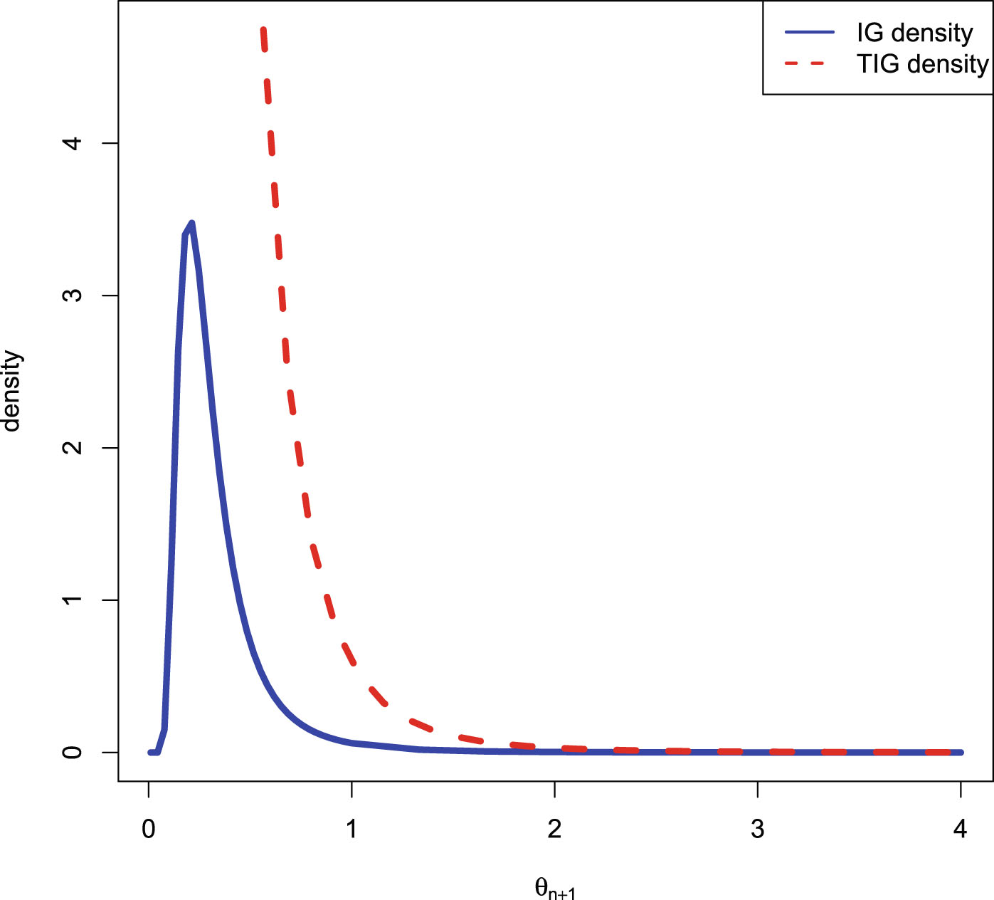
 and
and
 which exemplify the two inequalities (1.16) and (1.17).
and . Then we set a seed number 1 in R software (R Core Team (2023)) and draw from . After that, we draw from . Figure 7.1 shows the pdf of and the pdf of with , , and . From the figure, we see that the pdf of is left-peaked and right-skewed, and the pdf of is the pdf of truncated on . Numerical results show that
FIG. 7.1 — U-IG: The pdf of  and the pdf of
  with
with  ,
,  , and
, and  .
.
and the pdf of with , , and .
Now we allow one of the three quantities  ,
,  , and
, and  to change, holding other quantities fixed. In other words, we carry out sensitivity analyses of the Bayes estimators and the PESLs with respect to
  ,
,  , and
, and  . Figure 7.2 shows the Bayes estimators and the PESLs as functions of
  ,
,  , and
, and  . It is worth noting that the
  limits of the six plots are different. We see from the left plots of the figure that the Bayes estimators depend on
  ,
,  , and
, and  , and (1.16) is exemplified. More specifically, the Bayes estimators are decreasing functions of
  and
and  , while they are increasing functions of
  . The right plots of the figure exhibit that the PESLs also depend on
  ,
,  , and
, and  , and (1.17) is exemplified. More specifically, the PESLs are decreasing functions of
  ,
,  , and
, and  . Furthermore, tables 7.1–7.3 display the numerical values of the Bayes estimators and the PESLs in figure 7.2. In summary, the results of figure 7.2 and tables 7.1–7.3 exemplify the two inequalities (1.16) and (1.17).
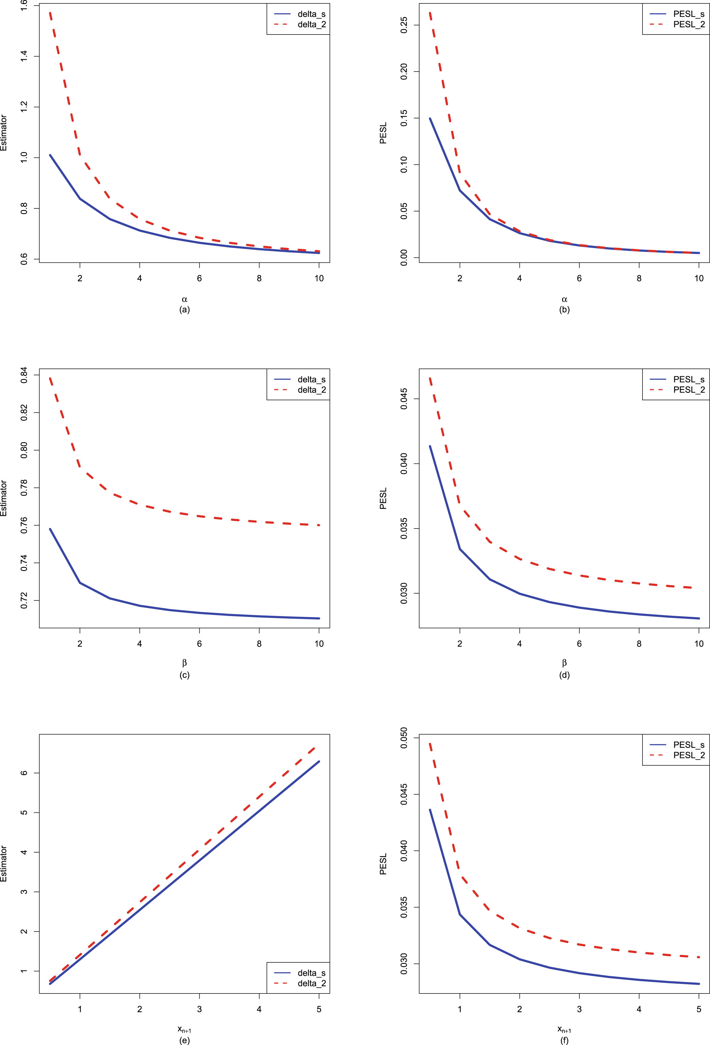
, , and to change, holding other quantities fixed. In other words, we carry out sensitivity analyses of the Bayes estimators and the PESLs with respect to , , and . Figure 7.2 shows the Bayes estimators and the PESLs as functions of , , and . It is worth noting that the limits of the six plots are different. We see from the left plots of the figure that the Bayes estimators depend on , , and , and (1.16) is exemplified. More specifically, the Bayes estimators are decreasing functions of and , while they are increasing functions of . The right plots of the figure exhibit that the PESLs also depend on , , and , and (1.17) is exemplified. More specifically, the PESLs are decreasing functions of , , and . Furthermore, tables 7.1–7.3 display the numerical values of the Bayes estimators and the PESLs in figure 7.2. In summary, the results of figure 7.2 and tables 7.1–7.3 exemplify the two inequalities (1.16) and (1.17).
FIG. 7.2 — U-IG: The Bayes estimators and the PESLs as functions of  ,
,  , and
, and  . (a) Bayes estimators vs.
  . (b) PESLs vs.
  . (c) Bayes estimators vs.
  . (d) PESLs vs.
  . (e) Bayes estimators vs.
  . (f) PESLs vs.
  .
.
, , and . (a) Bayes estimators vs. . (b) PESLs vs. . (c) Bayes estimators vs. . (d) PESLs vs. . (e) Bayes estimators vs. . (f) PESLs vs. .
TAB. 7.1 — U-IG: The numerical values of the Bayes estimators and the PESLs in figure 7.2:  changes.
changes.
 |
1 | 2 | 3 | 4 | 5 | 6 | 7 | 8 | 9 | 10 |
 |
1.0104 | 0.8382 | 0.7580 | 0.7128 | 0.6840 | 0.6644 | 0.6501 | 0.6393 | 0.6309 | 0.6242 |
 |
1.5708 | 1.0104 | 0.8382 | 0.7580 | 0.7128 | 0.6840 | 0.6644 | 0.6501 | 0.6393 | 0.6309 |
 |
0.1496 | 0.0722 | 0.0413 | 0.0263 | 0.0181 | 0.0131 | 0.0099 | 0.0077 | 0.0061 | 0.0050 |
 |
0.2629 | 0.0908 | 0.0466 | 0.0283 | 0.0189 | 0.0135 | 0.0101 | 0.0078 | 0.0062 | 0.0051 |
TAB. 7.2 — U-IG: The numerical values of the Bayes estimators and the PESLs in figure 7.2:  changes.
changes.
 |
1 | 2 | 3 | 4 | 5 | 6 | 7 | 8 | 9 | 10 |
 |
0.7580 | 0.7294 | 0.7211 | 0.7172 | 0.7149 | 0.7134 | 0.7123 | 0.7115 | 0.7109 | 0.7104 |
 |
0.8382 | 0.7908 | 0.7773 | 0.7709 | 0.7672 | 0.7648 | 0.7631 | 0.7618 | 0.7609 | 0.7601 |
 |
0.0413 | 0.0334 | 0.0311 | 0.0300 | 0.0293 | 0.0289 | 0.0286 | 0.0284 | 0.0282 | 0.0281 |
 |
0.0466 | 0.0368 | 0.0340 | 0.0326 | 0.0319 | 0.0314 | 0.0310 | 0.0308 | 0.0306 | 0.0304 |
TAB. 7.3 — U-IG: The numerical values of the Bayes estimators and the PESLs in figure 7.2:  changes.
changes.
 |
0.5 | 1 | 1.5 | 2 | 2.5 | 3 | 3.5 | 4 | 4.5 | 5 |
 |
0.6784 | 1.2971 | 1.9202 | 2.5443 | 3.1687 | 3.7934 | 4.4181 | 5.0429 | 5.6678 | 6.2927 |
 |
0.7543 | 1.4097 | 2.0729 | 2.7380 | 3.4037 | 4.0697 | 4.7359 | 5.4023 | 6.0687 | 6.7351 |
 |
0.0436 | 0.0344 | 0.0317 | 0.0304 | 0.0297 | 0.0292 | 0.0288 | 0.0286 | 0.0284 | 0.0282 |
 |
0.0495 | 0.0379 | 0.0347 | 0.0332 | 0.0323 | 0.0317 | 0.0313 | 0.0310 | 0.0308 | 0.0306 |
Since the Bayes estimators  and
and  and the PESLs
  and
and  depend on
  ,
,  , and
, and  , we can plot the surfaces of the differences of the Bayes estimators and the PESLs on the domain
  for
for  and 2 (other
  values can also be specified) via the R function persp3d() in the R package rgl (see Zhang et al. (2017, 2019b); Adler et al. (2017)). We remark that the R function persp3d() allows one to rotate the perspective plots of the surface according to one’s wishes. See figure 7.3. The domain for
  is
is  for all the plots. a is for
  and b is for
  in the axes of all the plots. From the left two plots, we see that
  for all
  on
on  for
for  and 2, which exemplifies (1.16). From the right two plots, we see that
  for all
  on
on  for
for  and 2, which exemplifies (1.17). The results of figure 7.3 exemplify the two inequalities (1.16) and (1.17).
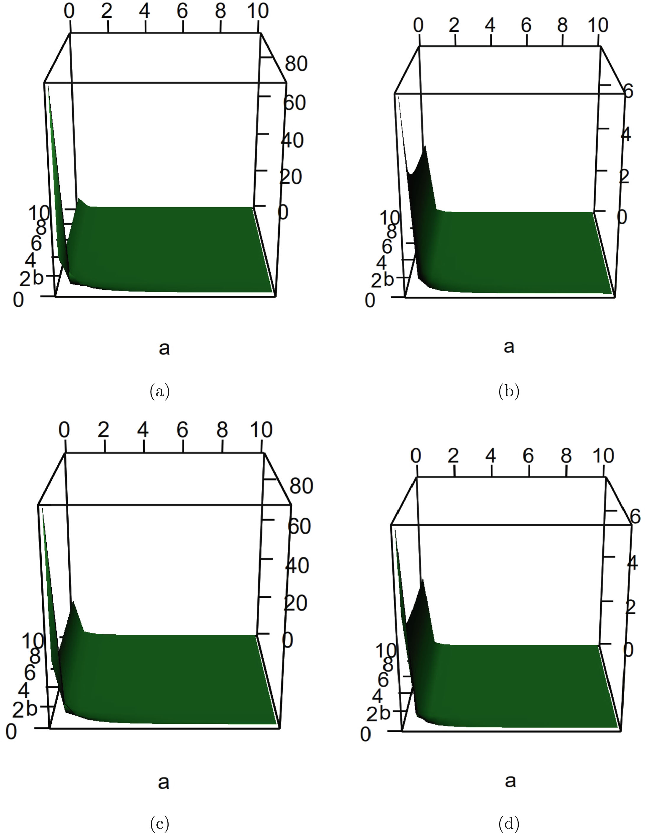
and and the PESLs and depend on , , and , we can plot the surfaces of the differences of the Bayes estimators and the PESLs on the domain for and 2 (other values can also be specified) via the R function persp3d() in the R package rgl (see Zhang et al. (2017, 2019b); Adler et al. (2017)). We remark that the R function persp3d() allows one to rotate the perspective plots of the surface according to one’s wishes. See figure 7.3. The domain for is for all the plots. a is for and b is for in the axes of all the plots. From the left two plots, we see that for all on for and 2, which exemplifies (1.16). From the right two plots, we see that for all on for and 2, which exemplifies (1.17). The results of figure 7.3 exemplify the two inequalities (1.16) and (1.17).
FIG. 7.3 — U-IG: (a) The surface of  which is positive for all
  on
on  for
for  . (b) The surface of
  which is positive for all
  on
on  for
for  . (c) The surface of
  which is positive for all
  on
on  for
for  . (d) The surface of
  which is positive for all
  on
on  for
for  .
.
which is positive for all on for . (b) The surface of which is positive for all on for . (c) The surface of which is positive for all on for . (d) The surface of which is positive for all on for .
7.3.2 Consistencies of the Moment Estimators and the MLEs
In this subsection, similar to subsection 1.8.1, we will numerically exemplify that the moment estimators ( ,
,  ) and the MLEs (
 ,
,  ) are consistent estimators of the hyperparameters (
 ,
,  ) of the hierarchical uniform and inverse gamma model (7.1). The motivation of this subsection is that in Theorems 7.2 and 7.3, we have theoretically shown that the moment estimators and the MLEs are consistent estimators of the hyperparameters. Note that only
  are used in this subsection.
, ) and the MLEs (, ) are consistent estimators of the hyperparameters (, ) of the hierarchical uniform and inverse gamma model (7.1). The motivation of this subsection is that in Theorems 7.2 and 7.3, we have theoretically shown that the moment estimators and the MLEs are consistent estimators of the hyperparameters. Note that only are used in this subsection.
The frequencies of the moment estimators ( ,
,  ) and the MLEs (
 ,
,  ) of the hyperparameters (
 ,
,  ) as
) as  varies for
  and
and  , 0.5, and 0.2 are reported in table 7.4. From the table, we observe the following facts.
, ) and the MLEs (, ) of the hyperparameters (, ) as varies for and , 0.5, and 0.2 are reported in table 7.4. From the table, we observe the following facts.
TAB. 7.4 — U-IG: The frequencies of the moment estimators and the MLEs of the hyperparameters as  varies for
  and
and  , 0.5, and 0.2.
varies for and , 0.5, and 0.2.
| Moment estimators | MLEs | ||||
 |
 |
 |
 |
 |
|
 |
200 | 0.27 | 0 | 0.09 | 0 |
| 400 | 0.15 | 0 | 0.01 | 0 | |
| 800 | 0.04 | 0 | 0 | 0 | |
| 1600 | 0.02 | 0 | 0 | 0 | |
 |
200 | 0.52 | 0.02 | 0.40 | 0.04 |
| 400 | 0.53 | 0 | 0.24 | 0 | |
| 800 | 0.33 | 0 | 0.04 | 0 | |
| 1600 | 0.21 | 0 | 0.02 | 0 | |
 |
200 | 0.85 | 0.54 | 0.74 | 0.45 |
| 400 | 0.80 | 0.52 | 0.62 | 0.25 | |
| 800 | 0.69 | 0.28 | 0.39 | 0.04 | |
| 1600 | 0.56 | 0.21 | 0.22 | 0 | |
1. Given  , 0.5, or 0.2, the frequencies of the estimators (
 ,
,  or
or  ,
,  ) tend to 0 as
  increases to infinity, which means that the moment estimators and the MLEs are consistent estimators of the hyperparameters. For
  , the frequencies of the estimators (
 ,
,  ,
,  ) are still very large (
 in all cases). However, we observe the tendencies of declining to 0 as
  increases to infinity.
, 0.5, or 0.2, the frequencies of the estimators (, or , ) tend to 0 as increases to infinity, which means that the moment estimators and the MLEs are consistent estimators of the hyperparameters. For , the frequencies of the estimators (, , ) are still very large ( in all cases). However, we observe the tendencies of declining to 0 as increases to infinity.
2. Comparing the frequencies corresponding to  , 0.5, and 0.2, we observe that as
  gets smaller, the frequencies tend to be larger, since the constraints
 (7.10)
, 0.5, and 0.2, we observe that as gets smaller, the frequencies tend to be larger, since the constraints
(7.10)
are easier to meet.
3. Theoretically, the consistency means that (1.22) for every  and every
  . However, we can only exemplify the limit (1.22) for several selected
  in simulations, for example,
  , 0.5, and 0.2. It is a reasonable setting, because as observed from this table when
  , the frequencies (
 ,
,  ,
,  ,
,  ) tend to 0 as
  tends to 1600. Moreover, when
  , the frequencies are getting bigger, since the constraints (7.10) are easier to meet, and the frequencies (
 ,
,  ,
,  ) still tend to 0 as
  tends to 1600. We observe the tendency of declining to 0 as
  increases to infinity for
  . Furthermore, when
  , the frequencies are getting even bigger, since the constraints (7.10) are easier to meet, and the frequency (
 ) still tends to 0 as
  tends to 1600. We observe the tendencies of declining to 0 as
  increases to infinity for the frequencies (
 ,
,  ,
,  ).
).
and every . However, we can only exemplify the limit (1.22) for several selected in simulations, for example, , 0.5, and 0.2. It is a reasonable setting, because as observed from this table when , the frequencies (, , , ) tend to 0 as tends to 1600. Moreover, when , the frequencies are getting bigger, since the constraints (7.10) are easier to meet, and the frequencies (, , ) still tend to 0 as tends to 1600. We observe the tendency of declining to 0 as increases to infinity for . Furthermore, when , the frequencies are getting even bigger, since the constraints (7.10) are easier to meet, and the frequency () still tends to 0 as tends to 1600. We observe the tendencies of declining to 0 as increases to infinity for the frequencies (, , ).
4. Comparing the moment estimators and the MLEs of the hyperparameters  and
and  , we see that the frequencies of the MLEs are smaller than those of the moment estimators (the frequencies corresponding to
  and
and  when estimating
  are exceptions), which means that the MLEs are better than the moment estimators when estimating the hyperparameters in terms of consistency.
and , we see that the frequencies of the MLEs are smaller than those of the moment estimators (the frequencies corresponding to and when estimating are exceptions), which means that the MLEs are better than the moment estimators when estimating the hyperparameters in terms of consistency.
5. An explanation to use  is given as follows. We originally set
  to calculate the frequencies. We use parallel computing with 20 cores, and in each core we compute 5 simulations. Hence, we have done
  simulations. However, 3 cores fail to obtain the MLEs of the hyperparameters due to the singularity of the matrix when
  . Therefore, we decided to calculate the frequencies through the available 85 (
 ) simulations.
is given as follows. We originally set to calculate the frequencies. We use parallel computing with 20 cores, and in each core we compute 5 simulations. Hence, we have done simulations. However, 3 cores fail to obtain the MLEs of the hyperparameters due to the singularity of the matrix when . Therefore, we decided to calculate the frequencies through the available 85 () simulations.
7.3.3 Goodness-of-Fit of the Model: KS Test
In this subsection, similar to subsection 1.8.2, we will calculate the goodness-of-fit of the hierarchical uniform and inverse gamma model (7.1) to the simulated data. The motivation of this subsection is that we want to check whether the marginal distribution of the hierarchical uniform and inverse gamma model (7.1) fits the simulated data well. Notice that only  are used in this subsection.
are used in this subsection.
In our problem, the null hypothesis specifies that
 where
where  is the marginal distribution of the hierarchical uniform and inverse gamma model (7.1). The marginal density of the
  distribution is given by (7.2) which is obviously one-dimensional continuous. Therefore, the KS test can be used as a measure of the goodness-of-fit.
is the marginal distribution of the hierarchical uniform and inverse gamma model (7.1). The marginal density of the distribution is given by (7.2) which is obviously one-dimensional continuous. Therefore, the KS test can be used as a measure of the goodness-of-fit.
The results of the KS test goodness-of-fit of the model (7.1) to the simulated data are reported in table 7.5. It is worth noting that the data are simulated according to the hierarchical uniform and inverse gamma model (7.1) with  and
and  . In the table, the hyperparameters
  and
and  are estimated by three methods. The first method is the oracle method, in that we know the hyperparameters
  and
and  . The second method is the moment method, in which the hyperparameters
  and
and  are estimated by their moment estimators (see Theorem 7.2). The third method is the MLE method, in which the hyperparameters
  and
and  are estimated by their MLEs (see Theorem 7.3). In the table, the sample size is
  , and the number of simulations is
  . Originally, we did 100 simulations. However, two simulations fail, because in the iteration process, the estimator of
  becomes negative and errors occur in the Matlab function Newtons().
and . In the table, the hyperparameters and are estimated by three methods. The first method is the oracle method, in that we know the hyperparameters and . The second method is the moment method, in which the hyperparameters and are estimated by their moment estimators (see Theorem 7.2). The third method is the MLE method, in which the hyperparameters and are estimated by their MLEs (see Theorem 7.3). In the table, the sample size is , and the number of simulations is . Originally, we did 100 simulations. However, two simulations fail, because in the iteration process, the estimator of becomes negative and errors occur in the Matlab function Newtons().
TAB. 7.5 — U-IG: The results of the KS test goodness-of-fit of the model (7.1) to the simulated data.
 |
 |
 |
|
 |
0.0224 | 0.0258 | 0.0162 |
 |
0.5025 | 0.3736 | 0.7950 |
 |
0.143 | 0.061 | 0.796 |
 |
0.143 | 0.061 | 0.796 |
 |
0.929 | 0.867 | 1.000 |
From table 7.5, we observe the following facts.
1. The  values for the three methods are respectively given by 0.0224, 0.0258, and 0.0162, which means that the MLE method is the best method, the oracle method is the second-best method, and the moment method is the worst method. A possible explanation for a phenomenon that the MLE method performs better than the oracle method is that in (1.23), the empirical cdf
  is based on data, and the population cdfs
  for the MLE method is also based on data, while the population cdf
  for the oracle method is not based on data.
values for the three methods are respectively given by 0.0224, 0.0258, and 0.0162, which means that the MLE method is the best method, the oracle method is the second-best method, and the moment method is the worst method. A possible explanation for a phenomenon that the MLE method performs better than the oracle method is that in (1.23), the empirical cdf is based on data, and the population cdfs for the MLE method is also based on data, while the population cdf for the oracle method is not based on data.
2. The  values for the three methods are respectively given by 0.5025, 0.3736, and 0.7950, which also means that the MLE method ranks first, the oracle method ranks second, and the moment method ranks third.
values for the three methods are respectively given by 0.5025, 0.3736, and 0.7950, which also means that the MLE method ranks first, the oracle method ranks second, and the moment method ranks third.
3. The  values for the three methods are respectively given by 0.143, 0.061, and 0.796. The
  value for the MLE method accounts for over half of the
  simulations. The order of preference for the three methods is the MLE method, the oracle method, and the moment method.
values for the three methods are respectively given by 0.143, 0.061, and 0.796. The value for the MLE method accounts for over half of the simulations. The order of preference for the three methods is the MLE method, the oracle method, and the moment method.
4. The  values for the three methods are respectively given by 0.143, 0.061, and 0.796. A small
  value corresponds to a large p-value. Therefore, the smallest
  value corresponds to the largest p-value. Hence, the
  value and the
  value for the three methods are the same. The order of preference for the three methods is the MLE method, the oracle method, and the moment method.
values for the three methods are respectively given by 0.143, 0.061, and 0.796. A small value corresponds to a large p-value. Therefore, the smallest value corresponds to the largest p-value. Hence, the value and the value for the three methods are the same. The order of preference for the three methods is the MLE method, the oracle method, and the moment method.
5. The  values for the three methods are respectively given by 0.929, 0.867, and 1.000. Once again, the order of preference for the three methods is the MLE method, the oracle method, and the moment method.
values for the three methods are respectively given by 0.929, 0.867, and 1.000. Once again, the order of preference for the three methods is the MLE method, the oracle method, and the moment method.
The boxplots of the  values and the p-values for the three methods are displayed in figure 7.4. From the figure, we observe the following facts.
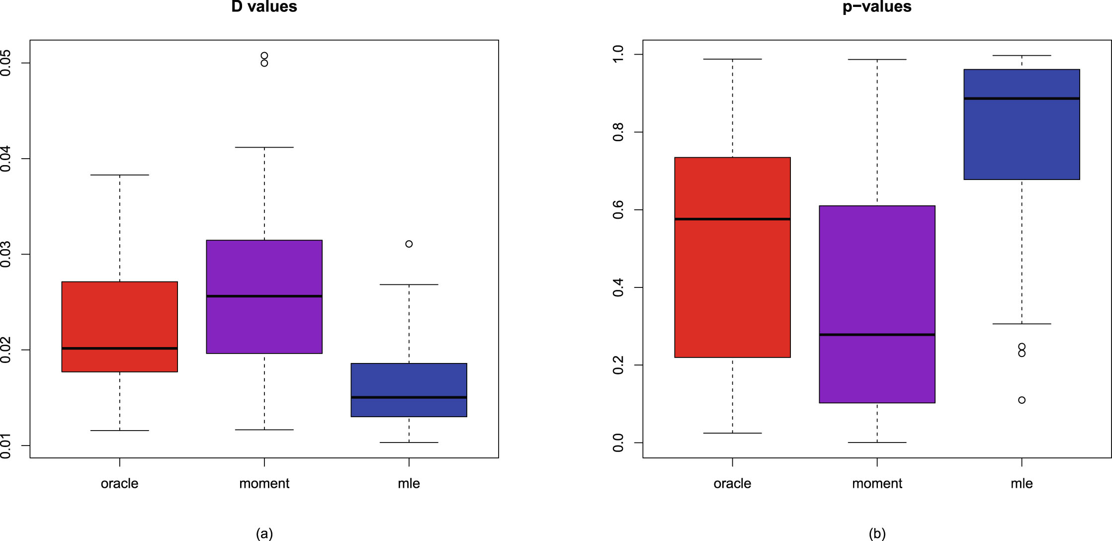
values and the p-values for the three methods are displayed in figure 7.4. From the figure, we observe the following facts.
FIG. 7.4 — U-IG: The boxplots of the  values and the p-values for the three methods. (a)
  values. (b) p-values.
values and the p-values for the three methods. (a) values. (b) p-values.
1. The  values of the moment method are significantly larger than those of the other two methods. For the
  value, the smaller the better. The order of preference for the three methods is the MLE method, the oracle method, and the moment method.
values of the moment method are significantly larger than those of the other two methods. For the value, the smaller the better. The order of preference for the three methods is the MLE method, the oracle method, and the moment method.
2. The p-values of the moment method are significantly smaller than those of the other two methods. For the p-value, the larger the better. The order of preference for the three methods is the MLE method, the oracle method, and the moment method.
3. Small  values correspond to large p-values, and large
  values correspond to small p-values.
values correspond to large p-values, and large values correspond to small p-values.
4. The MLE method has a better performance than the moment method in terms of the  values and the p-values.
values and the p-values.
7.3.4 Marginal Densities for Various Hyperparameters
In this subsection, we will plot the marginal densities of the hierarchical uniform and inverse gamma model (7.1) for various hyperparameters  and
and  . The motivation of this subsection is that we want to know what kind of data can be modeled by the hierarchical uniform and inverse gamma model (7.1). Note that the marginal density of
  is given by (7.2) specified by two hyperparameters
  and
and  . Note that
  is required to ensure that
 (7.11)
is positive. The derivation of (7.11) can be found in appendix A.25. It is easy to show that
(7.11)
is positive. The derivation of (7.11) can be found in appendix A.25. It is easy to show that  is a decreasing function of
  and
and  . Moreover, we will explore how the marginal densities change around the marginal density with hyperparameters specified by
  and
and  . Other numerical values of the hyperparameters can also be specified.
and . The motivation of this subsection is that we want to know what kind of data can be modeled by the hierarchical uniform and inverse gamma model (7.1). Note that the marginal density of is given by (7.2) specified by two hyperparameters and . Note that is required to ensure that
(7.11)
is a decreasing function of and . Moreover, we will explore how the marginal densities change around the marginal density with hyperparameters specified by and . Other numerical values of the hyperparameters can also be specified.
Figure 7.5 plots the marginal densities for varied  , holding
  fixed. From the figure we see that as
  increases, the peak value of the curve increases and the variance of the distribution decreases. Moreover, all the marginal densities are right-skewed.
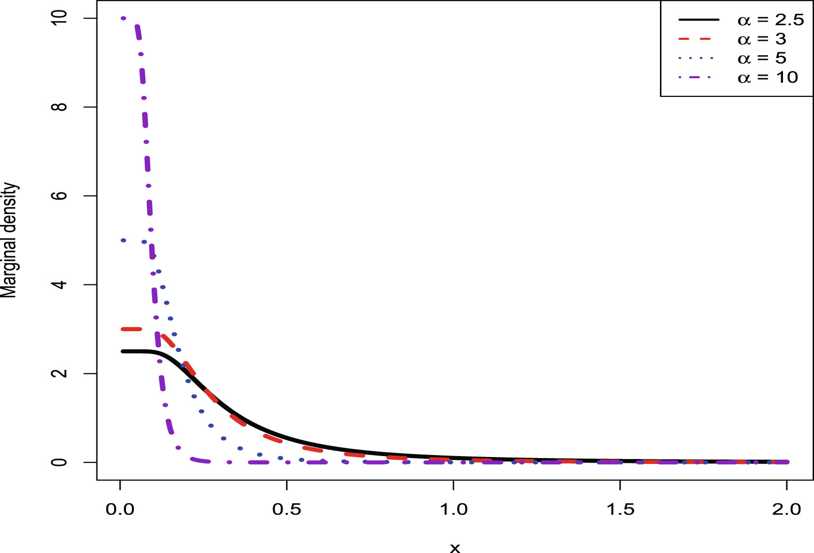
, holding fixed. From the figure we see that as increases, the peak value of the curve increases and the variance of the distribution decreases. Moreover, all the marginal densities are right-skewed.
FIG. 7.5 — U-IG: The marginal densities for varied  , holding
  fixed.
, holding fixed.
Figure 7.6 plots the marginal densities for varied  , holding
  fixed. From the figure, we also see that as
  increases, the peak value of the curve increases and the variance of the distribution decreases. Moreover, all the marginal densities are also right-skewed.
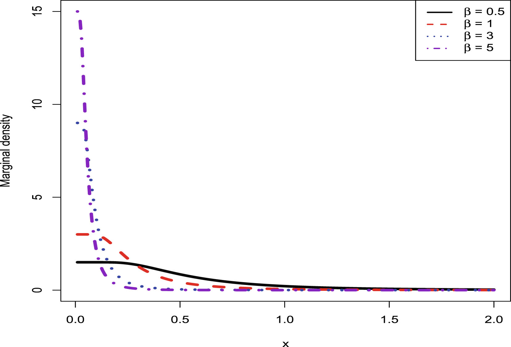
, holding fixed. From the figure, we also see that as increases, the peak value of the curve increases and the variance of the distribution decreases. Moreover, all the marginal densities are also right-skewed.
FIG. 7.6 — U-IG: The marginal densities for varied  , holding
  fixed.
, holding fixed.
7.4 A Real Data Example
In this section, we choose the current prices of the 300  component stocks of Shenzhen 300 Index on March 4, 2019, as the research objects. According to the proportion of the average circulating market value and the average turnover amount of 2:1 in a period of time, the stocks in the Shenzhen (a city in China) stock market rank from high to low. We select the top 300 stocks that constitute the initial component stocks of Shenzhen 300 Index. Shenzhen 300 Index is an indispensable reference for investors and securities practitioners to judge the trend of stock price change in the Shenzhen stock market.
component stocks of Shenzhen 300 Index on March 4, 2019, as the research objects. According to the proportion of the average circulating market value and the average turnover amount of 2:1 in a period of time, the stocks in the Shenzhen (a city in China) stock market rank from high to low. We select the top 300 stocks that constitute the initial component stocks of Shenzhen 300 Index. Shenzhen 300 Index is an indispensable reference for investors and securities practitioners to judge the trend of stock price change in the Shenzhen stock market.
It is worth mentioning that the original data  (the current prices of the 300 component stocks of Shenzhen 300 Index) do not have a good result of the goodness-of-fit of the model (7.1). However, the transformed data (the transformation is
  ,
,  ), henceforth the sample
  , behave well in terms of the goodness-of-fit of the model (7.1). The histograms of the original data
  and the sample
  are depicted in figure 7.7. From the figure, we see that the original data
  behave like count data, and the sample
  are right-skewed positive continuous data. It is worth noting that the supplementary information
  is used to estimate the hyperparameters and to compute the goodness-of-fit of the model, while the prime data
  is used in the computations of the Bayes estimators and PESLs.
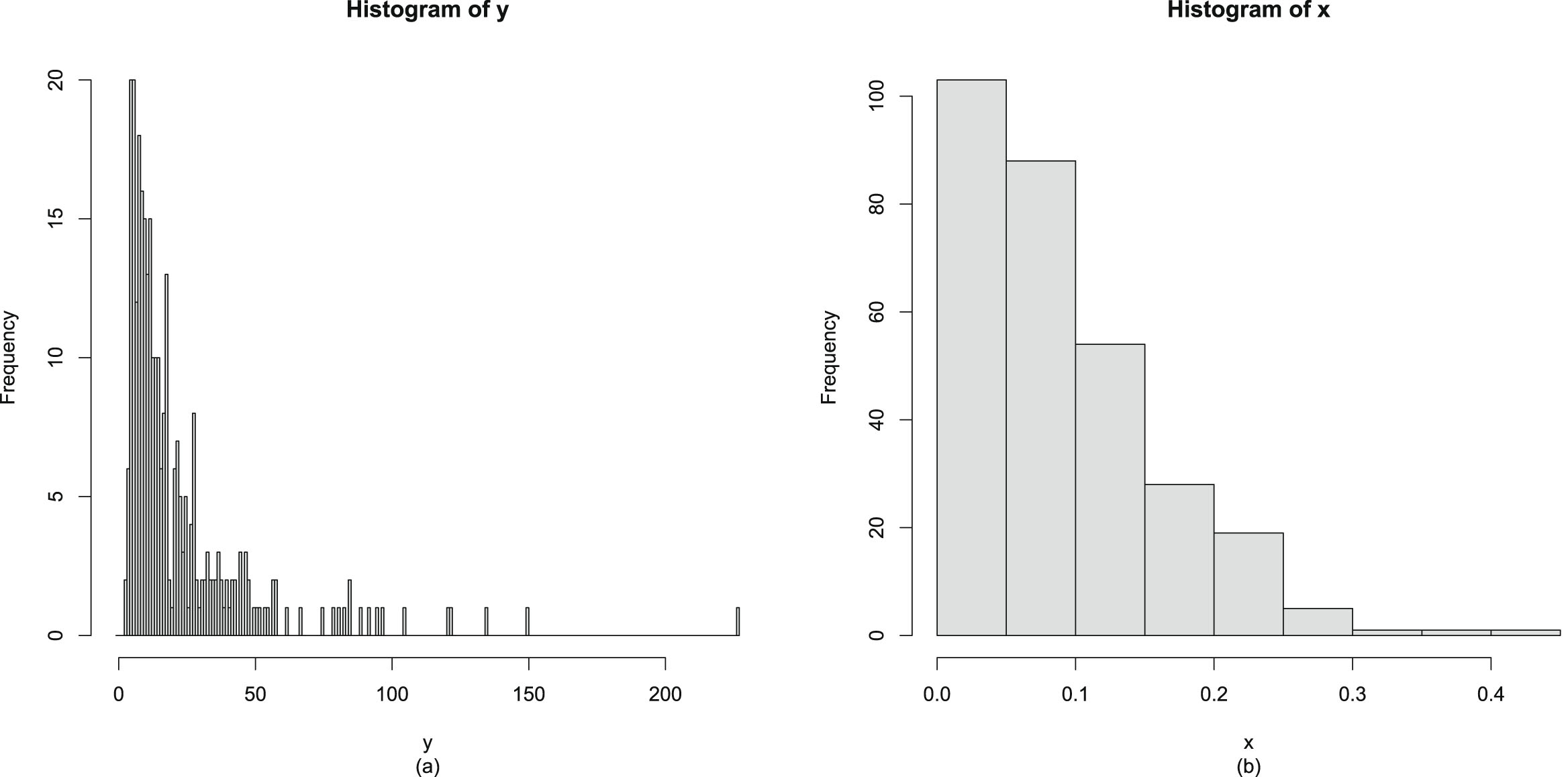
(the current prices of the 300 component stocks of Shenzhen 300 Index) do not have a good result of the goodness-of-fit of the model (7.1). However, the transformed data (the transformation is , ), henceforth the sample , behave well in terms of the goodness-of-fit of the model (7.1). The histograms of the original data and the sample are depicted in figure 7.7. From the figure, we see that the original data behave like count data, and the sample are right-skewed positive continuous data. It is worth noting that the supplementary information is used to estimate the hyperparameters and to compute the goodness-of-fit of the model, while the prime data is used in the computations of the Bayes estimators and PESLs.
FIG. 7.7 — U-IG: The histograms of the original data  and the sample
  . (a)
. (a)  . (b)
. (b)  .
.
and the sample . (a) . (b) .
The estimators of the hyperparameters  and
and  , the goodness-of-fit of the model, and the empirical Bayes estimators of the parameter of the uniform distribution with an inverse gamma prior and the PESLs by the moment method and the MLE method are summarized in table 7.6. From the table, we observe the following facts.
and , the goodness-of-fit of the model, and the empirical Bayes estimators of the parameter of the uniform distribution with an inverse gamma prior and the PESLs by the moment method and the MLE method are summarized in table 7.6. From the table, we observe the following facts.
TAB. 7.6 — U-IG: The estimators of the hyperparameters, the goodness-of-fit of the model, and the empirical Bayes estimators of the parameter of the uniform distribution with an inverse gamma prior and the PESLs by the moment method and the MLE method for the Shenzhen 300 Index.
| Moment method | MLE method | ||
| Estimators of the hyperparameters |  |
 |
 |
 |
 |
 |
|
| Goodness-of-fit of the model |  |
0.0501 | 0.0543 |
| p-value | 0.4399 | 0.3418 | |
| Empirical Bayes estimators and PESLs |  |
0.1438249 | 0.1347499 |
 |
0.1622345 | 0.1561949 | |
 |
0.0578093 | 0.0702162 | |
 |
0.0653631 | 0.0816789 |
1. The moment estimators and the MLEs of the hyperparameters  and
and  are quite different. This does not mean that the hierarchical uniform and inverse gamma model (7.1) does not fit the real data, nor mean that the moment estimators and the MLEs are not consistent estimators of the hyperparameters
  and
and  . The reason for the big differences between the two estimators is that the sample size
  is too small.
and are quite different. This does not mean that the hierarchical uniform and inverse gamma model (7.1) does not fit the real data, nor mean that the moment estimators and the MLEs are not consistent estimators of the hyperparameters and . The reason for the big differences between the two estimators is that the sample size is too small.
2. We use the KS test as a measure of the goodness-of-fit. The p-value of the moment method is  , and thus the
  distribution with
  and
and  estimated by their moment estimators, fits the sample
  well. Moreover, the p-value of the MLE method is
  , and thus the
  distribution with
  and
and  estimated by their MLEs fits the sample
  well. When comparing the two methods, we observe that the
  value of the moment method is smaller, and the p-value of the moment method is larger, which means that the
  distribution with
  and
and  estimated by the moment estimators has a better fit to the sample
  than that estimated by the MLEs. It is worth noting that the moment method could be better than the MLE method, as observed from table 7.5.
, and thus the distribution with and estimated by their moment estimators, fits the sample well. Moreover, the p-value of the MLE method is , and thus the distribution with and estimated by their MLEs fits the sample well. When comparing the two methods, we observe that the value of the moment method is smaller, and the p-value of the moment method is larger, which means that the distribution with and estimated by the moment estimators has a better fit to the sample than that estimated by the MLEs. It is worth noting that the moment method could be better than the MLE method, as observed from table 7.5.
3. When the hyperparameters are estimated by the moment method, we see that
 and
and

When the hyperparameters are estimated by the MLE method, we observe a similar phenomenon for the Bayes estimators and the PESLs. Consequently, the two inequalities (1.16) and (1.17) are exemplified.
7.5 Conclusions and Discussions
For the hierarchical uniform and inverse gamma model (7.1), we first calculate the posterior distribution of  ,
,  , and the marginal pdf of
  ,
,  , in Theorem 7.1. We then calculate the Bayes estimators
  and
and  , and the PESLs
  and
and  . Furthermore, they satisfy two inequalities (1.16) and (1.17). After that, the estimators of the hyperparameters of the model (7.1) by the moment method and their consistencies are summarized in Theorem 7.2. Moreover, the estimators of the hyperparameters of the model (7.1) by the MLE method and their consistencies are summarized in Theorem 7.3, whose proof involves the upper incomplete gamma function and its derivatives and a special case of the Meijer G-function and its derivatives. Finally, the empirical Bayes estimators of the parameter of the model (7.1) under Stein’s loss function by the moment method and the MLE method are summarized in Theorem 7.4.
, , and the marginal pdf of , , in Theorem 7.1. We then calculate the Bayes estimators and , and the PESLs and . Furthermore, they satisfy two inequalities (1.16) and (1.17). After that, the estimators of the hyperparameters of the model (7.1) by the moment method and their consistencies are summarized in Theorem 7.2. Moreover, the estimators of the hyperparameters of the model (7.1) by the MLE method and their consistencies are summarized in Theorem 7.3, whose proof involves the upper incomplete gamma function and its derivatives and a special case of the Meijer G-function and its derivatives. Finally, the empirical Bayes estimators of the parameter of the model (7.1) under Stein’s loss function by the moment method and the MLE method are summarized in Theorem 7.4.
We carry out the numerical simulations for the hierarchical uniform and inverse gamma model (7.1) in the simulations section. First, we have exemplified the two inequalities (1.16) and (1.17). After that, we have illustrated that the moment estimators and the MLEs are consistent estimators of the hyperparameters in table 7.4. Moreover, we have calculated the goodness-of-fit of the model (7.1) to the simulated data in table 7.5. Furthermore, the plots of the marginal densities show that all the curves are right-skewed. Therefore, the hierarchical uniform and inverse gamma model (7.1) could potentially be used to fit right-skewed positive continuous data instead of left-skewed positive continuous data. Finally, the estimators of the hyperparameters, the goodness-of-fit of the model, and the empirical Bayes estimators of the parameter of the uniform distribution with an inverse gamma prior and the PESLs by the moment method and the MLE method for the Shenzhen 300 Index are summarized in table 7.6.
To the best of our knowledge, there is no built-in or contributed R function which can deal with the Meijer G-function. Therefore, if one can contribute an R package which can deal with the Meijer G-function and its derivatives, then that would be very good news for the R community. Luckily, the meijerG() function introduced in Matlab R2017b can deal with the Meijer G-function, and hence our codes related to the Meijer G-function are written in Matlab. Consequently, our codes are a combination of R codes and Matlab codes.
When numerically computing
 where
where  is the numerator of
  and
and  is the denominator of
  , we get an NaN value as both
  and
and  are very small numbers that are close to 0. Moreover, we find that
  can be positive, negative, or 0, and
  is always positive. To overcome the numerical underflow problem, we compute
  as follows:
 where
where  is the sign of
  with
with

 is the absolute value of
  , and
, and  . After using the above technique, we obtain a finite value of
  .
.
is the numerator of and is the denominator of , we get an NaN value as both and are very small numbers that are close to 0. Moreover, we find that can be positive, negative, or 0, and is always positive. To overcome the numerical underflow problem, we compute as follows:
is the sign of with
is the absolute value of , and . After using the above technique, we obtain a finite value of .
Other things that need attention are the numerical computations of
 and
and
 where
where

Similar to the numerical computation of  , we encounter NaN values as
  ,
,  , and
, and  are all close to 0. To overcome the numerical underflow problem, we use the following technique:
 where
where

, we encounter NaN values as , , and are all close to 0. To overcome the numerical underflow problem, we use the following technique:
After using the above technique, we obtain finite values of  and
and  .
.
and .
It is worthy to point out that there exists an analytical solution to

The analytical calculations of  can be found in appendix A.27. However, there is a numerical accuracy problem with the above analytical solution. More specifically, the numerical integration by utilizing the R function integrate() produces a very small value of the magnitude of
  , while the analytical solution produces a not very small value of the magnitude of
  . Note that the denominator of
  is
is  which is a very small value of the magnitude of
  . Consequently, the numerical integration of
  gives us a reasonable value of
  of the magnitude of
  , while the analytical solution of
  gives us an unreasonably very large value of
  of the magnitude of
  . That is why we chose the numerical integration to compute
  .
.
can be found in appendix A.27. However, there is a numerical accuracy problem with the above analytical solution. More specifically, the numerical integration by utilizing the R function integrate() produces a very small value of the magnitude of , while the analytical solution produces a not very small value of the magnitude of . Note that the denominator of is which is a very small value of the magnitude of . Consequently, the numerical integration of gives us a reasonable value of of the magnitude of , while the analytical solution of gives us an unreasonably very large value of of the magnitude of . That is why we chose the numerical integration to compute .
Chapter 8 The Empirical Bayes Estimators of the Parameter of the Poisson Distribution with a Conjugate Gamma Prior under Stein’s Loss Function
For the hierarchical Poisson and gamma model, we calculate the Bayes estimator of the parameter of the Poisson distribution under Stein’s loss function, which penalizes gross overestimation and gross underestimation equally and the corresponding PESL. We also obtain the Bayes estimator of the parameter under the squared error loss function and the corresponding PESL. Moreover, we obtain the empirical Bayes estimators of the parameter of the Poisson distribution with a conjugate gamma prior by the moment method and the MLE method. In numerical simulations, we have illustrated four aspects: The two inequalities of the Bayes estimators and the PESLs; the consistencies of the moment estimators and the MLEs of the hyperparameters; the goodness-of-fit of the model to the simulated data; and the plots of the marginal probability mass functions (pmfs) for various hyperparameters. The numerical results indicate that the MLEs are better than the moment estimators when estimating the hyperparameters. Finally, we exploit the attendance data on 314 high school juniors from two urban high schools to illustrate our theoretical studies.
Acknowledgement. This chapter is derived in part from an article Zhang et al. (2019b) published in Journal of Statistical Computation and Simulation 08 August 2019 <Copyright Taylor & Francis>, available online: http://www.tandfonline.com/10.1080/00949655.2019.1652606.
8.1 Introduction
The hierarchical Poisson and gamma model (8.1) has been considered in exercise 4.32 (p. 196) of Casella and Berger (2002). It has been shown that the marginal distribution of  is a negative binomial distribution if
  is a positive integer. The Bayes estimation of
  , the parameter of the Poisson distribution, under the gamma prior is studied in Deely and Lindley (1981) and in tables 3.3.1 (p. 121) and 4.2.1 (p. 176) of Robert (2007). However, they only calculated the Bayes estimator of
  under the squared error loss function. Since
  is a positive parameter, the Bayes estimator of
  under the squared error loss function is not appropriate. In contrast, we should choose Stein’s loss function (James and Stein (1961); see also Brown (1990)) because it penalizes gross overestimation and gross underestimation equally. In this chapter, we calculate the Bayes estimator of
  under Stein’s loss function and the corresponding PESL. We also obtain the Bayes estimator of
  under the squared error loss function and the corresponding PESL. The Bayes estimators and the PESLs satisfy two inequalities (8.6) and (8.9). Moreover, we obtain the empirical Bayes estimators of the parameter of the Poisson distribution with a conjugate gamma prior by the moment method and the MLE method. Numerical simulations and a real data example illustrate our theoretical results.
is a negative binomial distribution if is a positive integer. The Bayes estimation of , the parameter of the Poisson distribution, under the gamma prior is studied in Deely and Lindley (1981) and in tables 3.3.1 (p. 121) and 4.2.1 (p. 176) of Robert (2007). However, they only calculated the Bayes estimator of under the squared error loss function. Since is a positive parameter, the Bayes estimator of under the squared error loss function is not appropriate. In contrast, we should choose Stein’s loss function (James and Stein (1961); see also Brown (1990)) because it penalizes gross overestimation and gross underestimation equally. In this chapter, we calculate the Bayes estimator of under Stein’s loss function and the corresponding PESL. We also obtain the Bayes estimator of under the squared error loss function and the corresponding PESL. The Bayes estimators and the PESLs satisfy two inequalities (8.6) and (8.9). Moreover, we obtain the empirical Bayes estimators of the parameter of the Poisson distribution with a conjugate gamma prior by the moment method and the MLE method. Numerical simulations and a real data example illustrate our theoretical results.
The rest of the chapter is organized as follows. In section 8.2, we calculate the Bayes estimators and the PESLs, and they satisfy two inequalities (8.6) and (8.9). Moreover, we summarize the empirical Bayes estimators of the parameter of the model (8.1) under Stein’s loss function by the moment method and the MLE method in Theorem 8.4. In section 8.3, we carry out some numerical simulations, where we have illustrated four aspects. First, we have exemplified the two inequalities (8.6) and (8.9). Second, we have illustrated that the moment estimators and the MLEs are consistent estimators of the hyperparameters. Third, we have calculated the goodness-of-fit of the model (8.1) to the simulated data. Finally, we have plotted the marginal pmfs of the model for various hyperparameters. A real data example is provided in section 8.4, where we exploit the attendance data on 314d high school juniors from two urban high schools, and the variable of interest is days absent. Some conclusions and discussions are provided in section 8.5.
8.2 Theoretical Results
Suppose that  are observed from the hierarchical Poisson and gamma model:
 (8.1)
where
(8.1)
where  and
and  are hyperparameters to be determined,
  is the unknown parameter of interest,
  is the Poisson distribution with an unknown mean
  , and
, and  is the gamma distribution with an unknown shape parameter
  and an unknown rate parameter
  . The gamma prior
  is a conjugate prior for the Poisson model, so that the posterior distribution of
  is also a gamma distribution. As described in Deely and Lindley (1981), the statistician observes data
  and wishes to make an inference about
  . Therefore,
  provides direct information about the parameter
  , while supplementary information
  is also available. The connection between the prime data
  and the supplementary information
  is provided by the common distributions
  and
and  . The pdfs of
  and
and  can be found in section 1.2.
are observed from the hierarchical Poisson and gamma model:
(8.1)
and are hyperparameters to be determined, is the unknown parameter of interest, is the Poisson distribution with an unknown mean , and is the gamma distribution with an unknown shape parameter and an unknown rate parameter . The gamma prior is a conjugate prior for the Poisson model, so that the posterior distribution of is also a gamma distribution. As described in Deely and Lindley (1981), the statistician observes data and wishes to make an inference about . Therefore, provides direct information about the parameter , while supplementary information is also available. The connection between the prime data and the supplementary information is provided by the common distributions and . The pdfs of and can be found in section 1.2.
8.2.1 The Bayes Estimators and the PESLs
For the hierarchical Poisson and gamma model (8.1), we have the following theorem which calculates the posterior density  and the marginal pmf
  . The proof of the theorem can be found in appendix A.28.
and the marginal pmf . The proof of the theorem can be found in appendix A.28.
Theorem 8.1. For the hierarchical Poisson and gamma model (8.1), the posterior density of  is a gamma distribution, that is,
 where
where
 (8.2)
(8.2)
is a gamma distribution, that is,
(8.2)
The marginal pmf of  is given by
 (8.3)
for
(8.3)
for  and
and  . In particular, when
  is a positive integer, the marginal distribution of
  is a negative binomial distribution,
  , with

is given by
(8.3)
and . In particular, when is a positive integer, the marginal distribution of is a negative binomial distribution, , with
Note that the particular part of Theorem 8.1 has been considered in exercise 4.32 (p. 196) of Casella and Berger (2002).
Now, let us analytically calculate the Bayes estimators  and
and  , and the PESLs
  and
and  under the hierarchical Poisson and gamma model (8.1) from (1.12)–(1.15). The three expectations are calculated as
 where
where  and
and  are given by (8.2). Now, let us calculate
  . For the sake of simplicity, the *’s are dropped from
  and
and  . We have
 where
where
 is the digamma function, which can be directly calculated in R software by digamma(x) (R Core Team (2023)). From (1.12), the Bayes estimator of
  under Stein’s loss function is given by
 (8.4)
for
(8.4)
for  . From (1.13), the Bayes estimator of
  under the usual squared error loss function is given by
 (8.5)
(8.5)
and , and the PESLs and under the hierarchical Poisson and gamma model (8.1) from (1.12)–(1.15). The three expectations are calculated as
and are given by (8.2). Now, let us calculate . For the sake of simplicity, the *’s are dropped from and . We have
under Stein’s loss function is given by
(8.4)
. From (1.13), the Bayes estimator of under the usual squared error loss function is given by
(8.5)
It is easy to show that
 (8.6)
which exemplifies the theoretical study of (1.16). Furthermore, from (1.14), the PESL at
(8.6)
which exemplifies the theoretical study of (1.16). Furthermore, from (1.14), the PESL at  is given by
 (8.7)
(8.7)
(8.6)
is given by
(8.7)
From (1.15), the PESL at  is given by
 (8.8)
(8.8)
is given by
(8.8)
It is easy to show that
 (8.9)
which exemplifies the theoretical study of (1.17). It is worth noting that the PESLs
(8.9)
which exemplifies the theoretical study of (1.17). It is worth noting that the PESLs  and
and  depend only on
  , but not on
  . Therefore, the PESLs depend only on
  and
and  , but not on
  .
.
(8.9)
and depend only on , but not on . Therefore, the PESLs depend only on and , but not on .
In the simulations section and the real data section, we will exemplify the two inequalities (8.6) and (8.9). Moreover, we will exemplify that the PESLs depend only on  and
and  , but not on
  .
.
and , but not on .
8.2.2 The Empirical Bayes Estimators of θn+1
The estimators of the hyperparameters of the model (8.1) by the moment method  and
and  and their consistencies are summarized in the following theorem whose proof can be found in appendix A.29.
and and their consistencies are summarized in the following theorem whose proof can be found in appendix A.29.
Theorem 8.2. The estimators of the hyperparameters of the model (8.1) by the moment method are
 (8.10)
 (8.11)
where
(8.11)
where
 is the sample
  th moment of
  . Moreover, the moment estimators are consistent estimators of the hyperparameters.
(8.10)
(8.11)
th moment of . Moreover, the moment estimators are consistent estimators of the hyperparameters.
The estimators of the hyperparameters of the model (8.1) by the MLE method  and
and  and their consistencies are summarized in the following theorem whose proof can be found in appendix A.30.
and and their consistencies are summarized in the following theorem whose proof can be found in appendix A.30.
Theorem 8.3. The estimators of the hyperparameters of the model (8.1) by the MLE method  and
and  are the solutions to the following equations:
 (8.12)
 (8.13)
and are the solutions to the following equations:
(8.12)
(8.13)
Moreover, the MLEs are consistent estimators of the hyperparameters.
The analytical calculations of the MLEs of  and
and  by solving the equations (8.12) and (8.13) are impossible, and thus we have to resort to numerical solutions. We can exploit Newton’s method to solve the equations (8.12) and (8.13), and to obtain the MLEs of
  and
and  . Note that the MLEs of
  and
and  are very sensitive to the initial estimators, and the moment estimators are usually proved to be good initial estimators.
and by solving the equations (8.12) and (8.13) are impossible, and thus we have to resort to numerical solutions. We can exploit Newton’s method to solve the equations (8.12) and (8.13), and to obtain the MLEs of and . Note that the MLEs of and are very sensitive to the initial estimators, and the moment estimators are usually proved to be good initial estimators.
Finally, the empirical Bayes estimators of the parameter of the model (8.1) under Stein’s loss function by the moment method and the MLE method are summarized in the following theorem.
Theorem 8.4. The empirical Bayes estimator of the parameter of the model (8.1) under Stein’s loss function by the moment method is given by (8.4) with the hyperparameters estimated by  in Theorem 8.2. Alternatively, the empirical Bayes estimator of the parameter of the model (8.1) under Stein’s loss function by the MLE method is given by (8.4) with the hyperparameters estimated by
  numerically determined in Theorem 8.3.
in Theorem 8.2. Alternatively, the empirical Bayes estimator of the parameter of the model (8.1) under Stein’s loss function by the MLE method is given by (8.4) with the hyperparameters estimated by numerically determined in Theorem 8.3.
8.3 Simulations
In this section, we will carry out the numerical simulations for the hierarchical Poisson and gamma model (8.1). We will illustrate four aspects. First, we will exemplify the two inequalities (8.6) and (8.9). Second, we will illustrate that the moment estimators and the MLEs are consistent estimators of the hyperparameters. Third, we will calculate the goodness-of-fit of the model (8.1) to the simulated data. Finally, we will plot the marginal pmfs of the model (8.1) for various hyperparameters.
The simulated data are generated according to the model (8.1) with the hyperparameters specified by  and
and  . The reason why we choose these values is that
  and
and  . Other numerical values of the hyperparameters can also be specified.
and . The reason why we choose these values is that and . Other numerical values of the hyperparameters can also be specified.
8.3.1 Two Inequalities of the Bayes Estimators and the PESLs
In this subsection, we will numerically exemplify the two inequalities of the Bayes estimators and the PESLs (8.6) and (8.9) for the oracle method. The motivation of this subsection is that theoretically we have the two inequalities (8.6) and (8.9).
First, we fix  and
and  . Then we set a seed number 1 in R software and draw
  from
from  . After that, we draw
  from
from  . Figure 8.1 shows the histogram of
  and the density estimation curve of
  . It is
  that we find
  to minimize the PESL. Numerical results show that
 and
and
 which exemplify the theoretical studies of (8.6) and (8.9).
and . Then we set a seed number 1 in R software and draw from . After that, we draw from . Figure 8.1 shows the histogram of and the density estimation curve of . It is that we find to minimize the PESL. Numerical results show that
Now we allow one of the three quantities  ,
,  , and
, and  to change, holding other quantities fixed. In other words, we are interested in the sensitivity analysis of the Bayes estimators and the PESLs about the three quantities
  ,
,  , and
, and  . Figure 8.2 shows the Bayes estimators and the PESLs as functions of
  ,
,  , and
, and  . We see from the left plots of the figure that the Bayes estimators depend on
  ,
,  , and
, and  , and (8.6) is exemplified. Moreover, the Bayes estimators are increasing functions of
  and
and  , and they are decreasing functions of
  . The right plots of the figure exhibit that the PESLs depend only on
  and
and  , but not on
  , and (8.9) is exemplified. In addition, the PESLs are decreasing functions of
  and
and  . Furthermore, tables 8.1–8.3 display the numerical values of the Bayes estimators and the PESLs in Figure 8.2. In summary, the results of figure 8.2 and tables 8.1–8.3 exemplify the two inequalities (8.6) and (8.9).
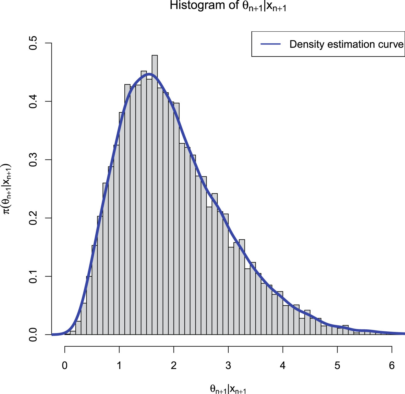
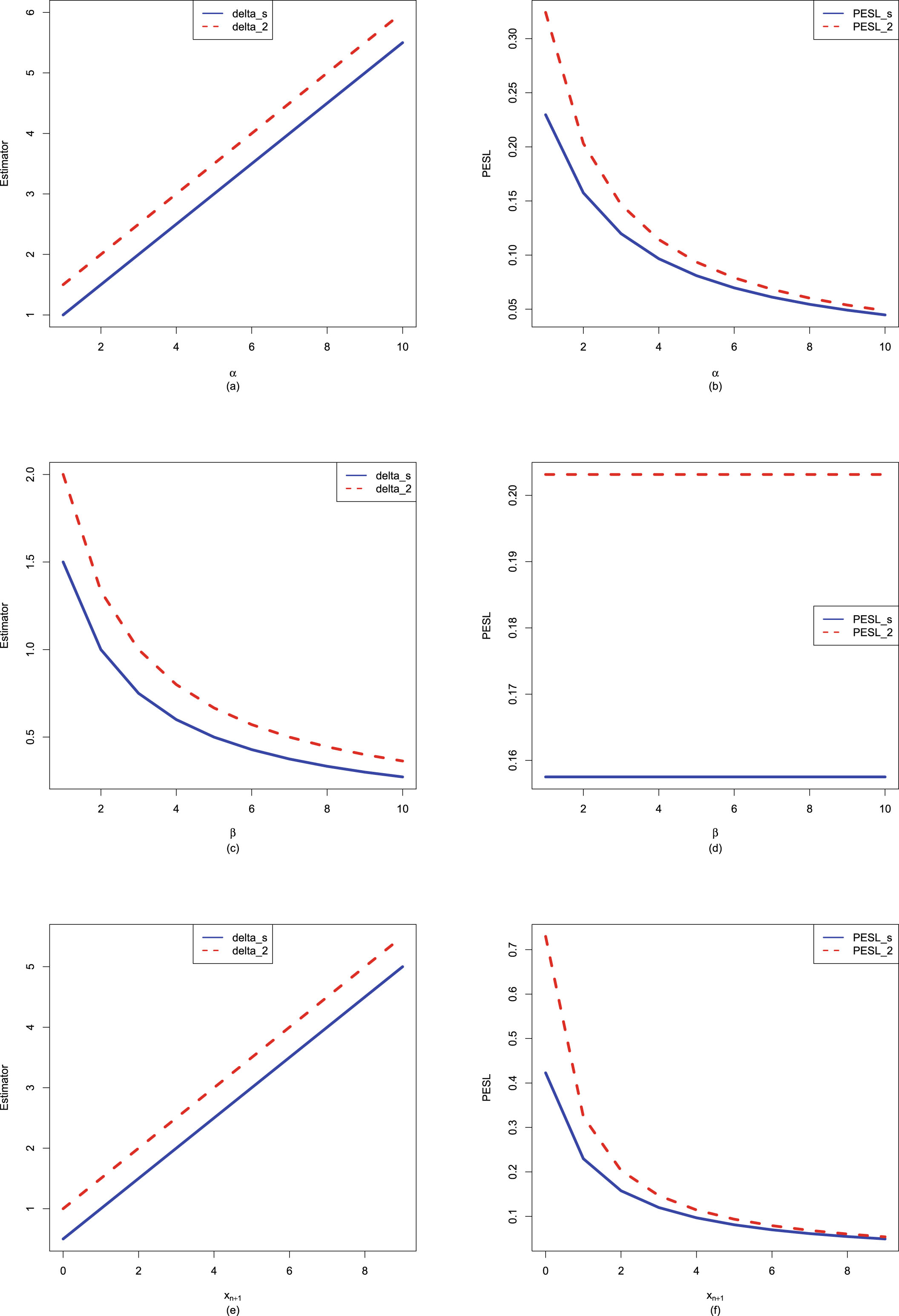
, , and to change, holding other quantities fixed. In other words, we are interested in the sensitivity analysis of the Bayes estimators and the PESLs about the three quantities , , and . Figure 8.2 shows the Bayes estimators and the PESLs as functions of , , and . We see from the left plots of the figure that the Bayes estimators depend on , , and , and (8.6) is exemplified. Moreover, the Bayes estimators are increasing functions of and , and they are decreasing functions of . The right plots of the figure exhibit that the PESLs depend only on and , but not on , and (8.9) is exemplified. In addition, the PESLs are decreasing functions of and . Furthermore, tables 8.1–8.3 display the numerical values of the Bayes estimators and the PESLs in Figure 8.2. In summary, the results of figure 8.2 and tables 8.1–8.3 exemplify the two inequalities (8.6) and (8.9).
FIG. 8.1 — P-G: The histogram of  and the density estimation curve of
  .
.
and the density estimation curve of .
FIG. 8.2 — P-G: The Bayes estimators and the PESLs as functions of  ,
,  , and
, and  . (a), (c), (e) Bayes estimators vs.
  ,
,  , and
, and  . (b), (d), (f) PESLs vs.
  ,
,  , and
, and  .
.
, , and . (a), (c), (e) Bayes estimators vs. , , and . (b), (d), (f) PESLs vs. , , and .
TAB. 8.1 — P-G: The numerical values of the Bayes estimators and the PESLs in figure 8.2:  changes.
changes.
 |
1 | 2 | 3 | 4 | 5 | 6 | 7 | 8 | 9 | 10 |
 |
1.0000 | 1.5000 | 2.0000 | 2.5000 | 3.0000 | 3.5000 | 4.0000 | 4.5000 | 5.0000 | 5.5000 |
 |
1.5000 | 2.0000 | 2.5000 | 3.0000 | 3.5000 | 4.0000 | 4.5000 | 5.0000 | 5.5000 | 6.0000 |
 |
0.2296 | 0.1575 | 0.1198 | 0.0967 | 0.0810 | 0.0697 | 0.0612 | 0.0545 | 0.0492 | 0.0448 |
 |
0.3242 | 0.2032 | 0.1467 | 0.1144 | 0.0935 | 0.0791 | 0.0684 | 0.0603 | 0.0539 | 0.0487 |
TAB. 8.2 — P-G: The numerical values of the Bayes estimators and the PESLs in figure 8.2:  changes.
changes.
 |
1 | 2 | 3 | 4 | 5 | 6 | 7 | 8 | 9 | 10 |
 |
1.5000 | 1.0000 | 0.7500 | 0.6000 | 0.5000 | 0.4286 | 0.3750 | 0.3333 | 0.3000 | 0.2727 |
 |
2.0000 | 1.3333 | 1.0000 | 0.8000 | 0.6667 | 0.5714 | 0.5000 | 0.4444 | 0.4000 | 0.3636 |
 |
0.1575 | 0.1575 | 0.1575 | 0.1575 | 0.1575 | 0.1575 | 0.1575 | 0.1575 | 0.1575 | 0.1575 |
 |
0.2032 | 0.2032 | 0.2032 | 0.2032 | 0.2032 | 0.2032 | 0.2032 | 0.2032 | 0.2032 | 0.2032 |
TAB. 8.3 — P-G: The numerical values of the Bayes estimators and the PESLs in figure 8.2:  changes.
changes.
 |
0 | 1 | 2 | 3 | 4 | 5 | 6 | 7 | 8 | 9 |
 |
0.5000 | 1.0000 | 1.5000 | 2.0000 | 2.5000 | 3.0000 | 3.5000 | 4.0000 | 4.5000 | 5.0000 |
 |
1.0000 | 1.5000 | 2.0000 | 2.5000 | 3.0000 | 3.5000 | 4.0000 | 4.5000 | 5.0000 | 5.5000 |
 |
0.4228 | 0.2296 | 0.1575 | 0.1198 | 0.0967 | 0.0810 | 0.0697 | 0.0612 | 0.0545 | 0.0492 |
 |
0.7296 | 0.3242 | 0.2032 | 0.1467 | 0.1144 | 0.0935 | 0.0791 | 0.0684 | 0.0603 | 0.0539 |
Since the Bayes estimators  and
and  and the PESLs
  and
and  depend on
  and
and  , where
  and
and  , we can plot the surfaces of the Bayes estimators and the PESLs on the domain
  via the R function persp3d() in the R package rgl (see Sun et al. (2021); Zhang et al. (2017, 2019b); Adler et al. (2017)). We remark that the R function persp() in the R package graphics can not add another surface to the existing surface, but persp3d() can. Moreover, persp3d() allows one to rotate the perspective plots of the surface according to one’s wishes. Figure 8.3 plots the surfaces of the Bayes estimators and the PESLs, and the surfaces of the differences of the Bayes estimators and the PESLs. The domain for
  is
is  for all the plots. a is for
  and b is for
  in the axes of all the plots. The red surface is for
  and the blue surface is for
  in the upper two plots. From the left two plots of the figure, we see that
  for all
  on
on  , which exemplifies (8.6). From the right two plots of the figure, we see that
  for all
  on
on  , which exemplifies (8.9). The results of the figure exemplify the theoretical studies of (8.6) and (8.9).
and and the PESLs and depend on and , where and , we can plot the surfaces of the Bayes estimators and the PESLs on the domain via the R function persp3d() in the R package rgl (see Sun et al. (2021); Zhang et al. (2017, 2019b); Adler et al. (2017)). We remark that the R function persp() in the R package graphics can not add another surface to the existing surface, but persp3d() can. Moreover, persp3d() allows one to rotate the perspective plots of the surface according to one’s wishes. Figure 8.3 plots the surfaces of the Bayes estimators and the PESLs, and the surfaces of the differences of the Bayes estimators and the PESLs. The domain for is for all the plots. a is for and b is for in the axes of all the plots. The red surface is for and the blue surface is for in the upper two plots. From the left two plots of the figure, we see that for all on , which exemplifies (8.6). From the right two plots of the figure, we see that for all on , which exemplifies (8.9). The results of the figure exemplify the theoretical studies of (8.6) and (8.9).
8.3.2 Consistencies of the Moment Estimators and the MLEs
In this subsection, similar to subsection 1.8.1, we will numerically exemplify that the moment estimators ( ,
,  ) and the MLEs (
 ,
,  ) are consistent estimators of the hyperparameters (
 ,
,  ) of the hierarchical Poisson and gamma model (8.1). The motivation of this subsection is that in Theorems 8.2 and 8.3, we have theoretically shown that the moment estimators and the MLEs are consistent estimators of the hyperparameters. Note that only
  are used in this subsection.
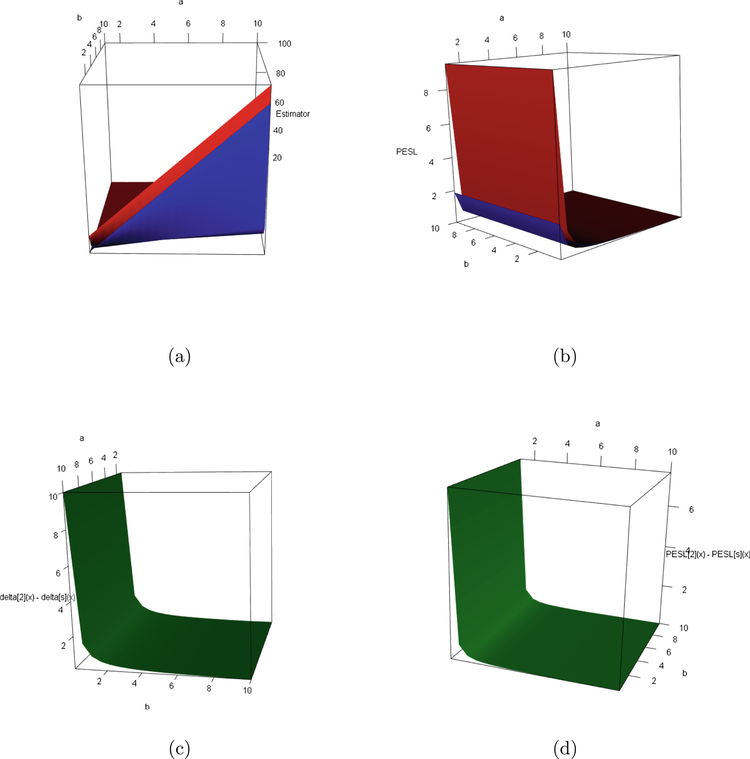
, ) and the MLEs (, ) are consistent estimators of the hyperparameters (, ) of the hierarchical Poisson and gamma model (8.1). The motivation of this subsection is that in Theorems 8.2 and 8.3, we have theoretically shown that the moment estimators and the MLEs are consistent estimators of the hyperparameters. Note that only are used in this subsection.
FIG. 8.3 — P-G: (a) The Bayes estimators as functions of  and
and  . (b) The PESLs as functions of
  and
and  . (c) The surface of
  which is positive for all
  on
on  . (d) The surface of
  which is also positive for all
  on
on  .
.
and . (b) The PESLs as functions of and . (c) The surface of which is positive for all on . (d) The surface of which is also positive for all on .
The frequencies of the moment estimators ( ,
,  ) and the MLEs (
 ,
,  ) of the hyperparameters (
 ,
,  ) as
) as  varies for
  and
and  , 0.5, and 0.1 are reported in table 8.4. From the table, we observe the following facts.
, ) and the MLEs (, ) of the hyperparameters (, ) as varies for and , 0.5, and 0.1 are reported in table 8.4. From the table, we observe the following facts.
1. Given  , 0.5, or 0.1, the frequencies of the estimators (
 ,
,  ,
,  ,
,  ) tend to 0 as
  increases to infinity, which means that the moment estimators and the MLEs are consistent estimators of the hyperparameters. For
  , the frequencies of the estimators
  and
and  are still very large (
 for all the cases). However, we observe the tendencies of declining to 0 as
  increases to infinity.
, 0.5, or 0.1, the frequencies of the estimators (, , , ) tend to 0 as increases to infinity, which means that the moment estimators and the MLEs are consistent estimators of the hyperparameters. For , the frequencies of the estimators and are still very large ( for all the cases). However, we observe the tendencies of declining to 0 as increases to infinity.
2. Comparing the frequencies corresponding to  , 0.5, and 0.1, we observe that as
  gets smaller, the frequencies tend to be larger, since the constraints

, 0.5, and 0.1, we observe that as gets smaller, the frequencies tend to be larger, since the constraints
are easier to meet.
3. Comparing the moment estimators and the MLEs of the hyperparameters  and
and  , we see that the frequencies of the MLEs are smaller than those of the moment estimators for large
  , which means that the MLEs are better than the moment estimators when estimating the hyperparameters in terms of consistency.
and , we see that the frequencies of the MLEs are smaller than those of the moment estimators for large , which means that the MLEs are better than the moment estimators when estimating the hyperparameters in terms of consistency.
8.3.3 Goodness-of-Fit of the Model: Chi-Square Test
In this subsection, similar to subsection 1.8.2, we will calculate the goodness-of-fit of the hierarchical Poisson and gamma model (8.1) to the simulated data. The motivation of this subsection is that we want to check whether the marginal distribution of the hierarchical Poisson and gamma model (8.1) fits the simulated data well. Note that only  are used in this subsection.
are used in this subsection.
TAB. 8.4 — P-G: The frequencies of the moment estimators and the MLEs of the hyperparameters as  varies for
  and
and  , 0.5, and 0.1.
varies for and , 0.5, and 0.1.
| Moment estimators | MLEs | ||||
 |
 |
 |
 |
 |
|
 |
1e3 | 0 | 0 | 0 | 0 |
| 2e3 | 0 | 0 | 0 | 0 | |
| 4e3 | 0 | 0 | 0 | 0 | |
| 8e3 | 0 | 0 | 0 | 0 | |
 |
1e3 | 0.06 | 0 | 0.01 | 0 |
| 2e3 | 0 | 0 | 0 | 0 | |
| 4e3 | 0 | 0 | 0 | 0 | |
| 8e3 | 0 | 0 | 0 | 0 | |
 |
1e3 | 0.65 | 0.39 | 0.67 | 0.40 |
| 2e3 | 0.56 | 0.24 | 0.48 | 0.24 | |
| 4e3 | 0.41 | 0.12 | 0.31 | 0.09 | |
| 8e3 | 0.22 | 0.03 | 0.17 | 0 | |
The results of the goodness-of-fit of the model (8.1) to the simulated data are reported in table 8.5. Note that the data is simulated according to the hierarchical Poisson and gamma model (8.1) with  and
and  . In the table,
  is the number of groups,
  is the sample size,
  is the chi-square statistic, which is equal to
  or
or  in the first or second case, respectively,
  is the degree of freedom of the limiting chi-square distribution, and the p-value is the probability that a value of
  as large as the one observed would have occurred if the null hypothesis were true. From the table, we observe the following facts.
and . In the table, is the number of groups, is the sample size, is the chi-square statistic, which is equal to or in the first or second case, respectively, is the degree of freedom of the limiting chi-square distribution, and the p-value is the probability that a value of as large as the one observed would have occurred if the null hypothesis were true. From the table, we observe the following facts.
1. In the first column of the table, the null hypothesis is

where  is the marginal distribution of the hierarchical Poisson and gamma model (8.1) with
  and
and  known, and thus
  . The p-value
  , and thus the
  distribution with
  and
and  fits the simulated data well.
is the marginal distribution of the hierarchical Poisson and gamma model (8.1) with and known, and thus . The p-value , and thus the distribution with and fits the simulated data well.
2. In the second column of the table, the null hypothesis specifies that  is distributed to a
  distribution with
  and
and  unknown. The unknown hyperparameters
  and
and  are estimated by their moment estimators
  and
and  based on the simulated sample with a sample size
  . Therefore, the
  . The p-value
  , and thus the
  distribution with
  and
and  estimated by their moment estimators fits the simulated data well.
is distributed to a distribution with and unknown. The unknown hyperparameters and are estimated by their moment estimators and based on the simulated sample with a sample size . Therefore, the . The p-value , and thus the distribution with and estimated by their moment estimators fits the simulated data well.
3. In the third column of the table, the null hypothesis specifies that  is distributed to a
  distribution with
  and
and  unknown. The unknown hyperparameters
  and
and  are estimated by the MLEs
  and
and  based on the simulated sample with a sample size
  . Therefore, the
  . The p-value
  , and thus the
  distribution with
  and
and  estimated by their MLEs fits the simulated data well.
is distributed to a distribution with and unknown. The unknown hyperparameters and are estimated by the MLEs and based on the simulated sample with a sample size . Therefore, the . The p-value , and thus the distribution with and estimated by their MLEs fits the simulated data well.
4. Comparing the second and third columns to the first column of the table, we find that the degree of freedom is lost by 2, and the p-value is increased. Nevertheless, all the columns indicate that the hierarchical Poisson and gamma model (8.1) fits the simulated data well.
5. Comparing the second column to the third column of the table, we see that the degrees of freedom are the same, the  value of the MLEs is smaller, and the p-value of the MLEs is larger, which means that the
  distribution with the hyperparameters
  and
and  estimated by the MLEs has a better fit to the simulated data than that estimated by the moment estimators.
value of the MLEs is smaller, and the p-value of the MLEs is larger, which means that the distribution with the hyperparameters and estimated by the MLEs has a better fit to the simulated data than that estimated by the moment estimators.
TAB. 8.5 — P-G: The results of the goodness-of-fit of the model (8.1) to the simulated data.
 |
 |
 |
|
 |
10 | 10 | 10 |
 |
 |
 |
 |
 |
11.011 | 8.679 | 7.600 |
 |
9 | 7 | 7 |
| p-value | 0.275 | 0.277 | 0.369 |
8.3.4 Marginal pmfs for Various Hyperparameters
In this subsection, we will plot the marginal pmfs of the hierarchical Poisson and gamma model (8.1) for various hyperparameters  and
and  . The motivation of this subsection is that we want to know what kind of data can be modeled by the hierarchical Poisson and gamma model (8.1). Note that the marginal pmf of
  is given by (8.3) specified by two hyperparameters
  and
and  . We will explore how the marginal pmfs change around the marginal pmf with hyperparameters specified by
  and
and  . Other numerical values of the hyperparameters can also be specified.
and . The motivation of this subsection is that we want to know what kind of data can be modeled by the hierarchical Poisson and gamma model (8.1). Note that the marginal pmf of is given by (8.3) specified by two hyperparameters and . We will explore how the marginal pmfs change around the marginal pmf with hyperparameters specified by and . Other numerical values of the hyperparameters can also be specified.
Figure 8.4 plots the marginal pmfs for varied  , holding
  fixed. From the figure, we see that as
  increases, the peak value of the marginal pmf decreases. In other words, the variance of the marginal pmf increases as
 (8.14)
is an increasing function of
(8.14)
is an increasing function of  . Moreover, the peak is shifted to the right. In addition, the sum of the marginal pmfs for
  for
for  are respectively computed as

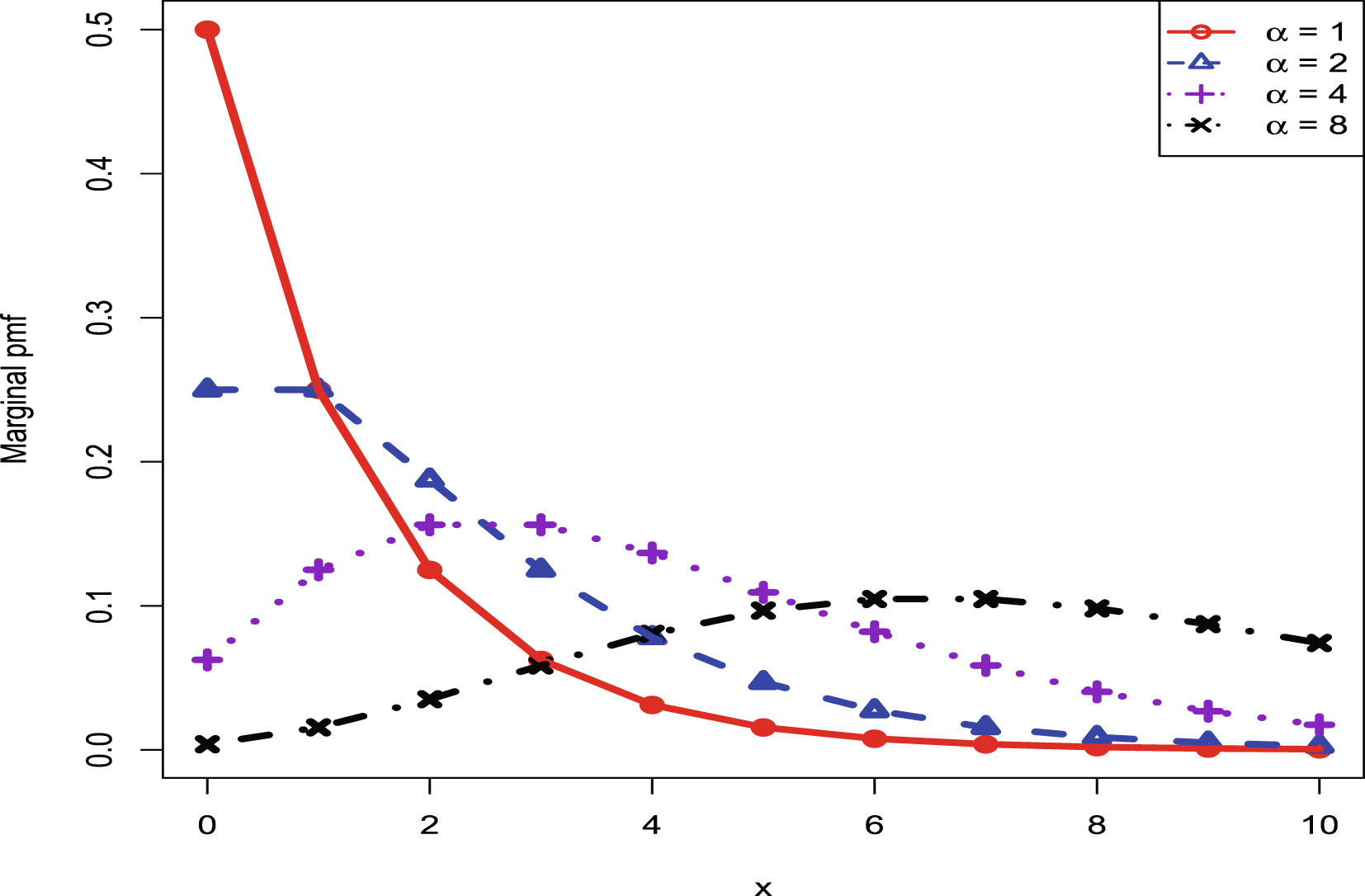
, holding fixed. From the figure, we see that as increases, the peak value of the marginal pmf decreases. In other words, the variance of the marginal pmf increases as
(8.14)
. Moreover, the peak is shifted to the right. In addition, the sum of the marginal pmfs for for are respectively computed as
FIG. 8.4 — P-G: The marginal pmfs for varied  , holding
  fixed.
, holding fixed.
We observe that as  increases, the sum of the marginal pmfs for
  decreases.
increases, the sum of the marginal pmfs for decreases.
Figure 8.5 plots the marginal pmfs for varied  , holding
  fixed. From the figure, we see that as
  increases, the peak value of the marginal pmf increases. In other words, the variance of the marginal pmf decreases, as (8.14) is a decreasing function of
  . Moreover, the peak is shifted to the left. In addition, the sum of the marginal pmfs for
  for
for  are respectively computed as

, holding fixed. From the figure, we see that as increases, the peak value of the marginal pmf increases. In other words, the variance of the marginal pmf decreases, as (8.14) is a decreasing function of . Moreover, the peak is shifted to the left. In addition, the sum of the marginal pmfs for for are respectively computed as
We observe that as  increases, the sum of the marginal pmfs for
  increases.
increases, the sum of the marginal pmfs for increases.
It is important to point out that the marginal pmfs only take values on 0 and positive integers. They are equal to 0 at other points. The lines in figures 8.4 and 8.5 are used to indicate tendencies of the marginal pmfs, not for the values of the marginal pmfs.
8.4 A Real Data Example
In this section, we exploit the attendance data on  high school juniors from two urban high schools in the file nb_data (see UCLA Institute for Digital Research and Education (2018)). The variable of interest
  is days absent, daysabs.
high school juniors from two urban high schools in the file nb_data (see UCLA Institute for Digital Research and Education (2018)). The variable of interest is days absent, daysabs.
The sample unconditional mean and variance of  and
and  are summarized in table 8.6. From the table, we observe that the sample unconditional mean of our outcome variable is much lower than its variance, and thus a Poisson model is not appropriate. We will see in the following that the hierarchical Poisson and gamma model (8.1) fits the data very well.
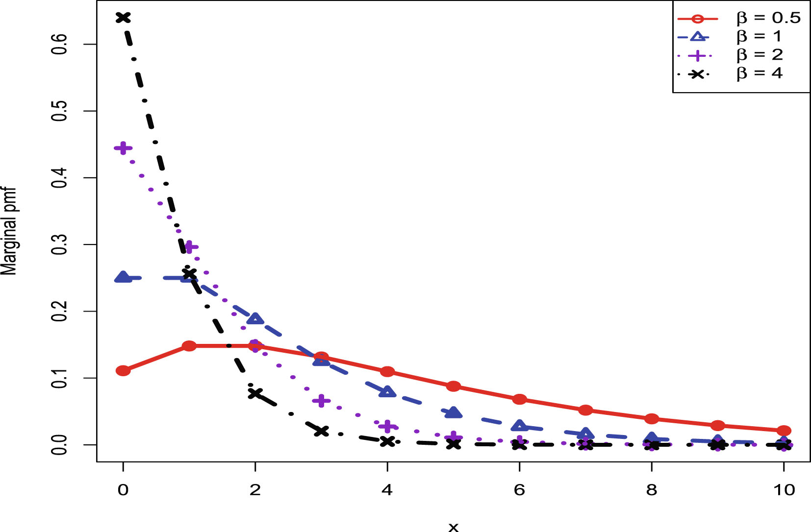
and are summarized in table 8.6. From the table, we observe that the sample unconditional mean of our outcome variable is much lower than its variance, and thus a Poisson model is not appropriate. We will see in the following that the hierarchical Poisson and gamma model (8.1) fits the data very well.
FIG. 8.5 — P-G: The marginal pmfs for varied  , holding
  fixed.
, holding fixed.
TAB. 8.6 — P-G: The sample unconditional mean and variance of  and
and  .
.
and .
 |
 |
|
 |
5.968 | 5.955 |
 |
49.627 | 49.519 |
Note that  with
with  .
.  is used in the goodness-of-fit of the model to the data.
with . is used in the goodness-of-fit of the model to the data.
The frequencies of  are summarized in table 8.7.
are summarized in table 8.7.
TAB. 8.7 — P-G: The frequencies of  .
.
.
| Value | 0 | 1 | 2 | 3 | 4 | 5 | 6 | 7 | 8 | 9 | 10 | 11 |
| Frequency | 57 | 41 | 27 | 27 | 25 | 20 | 16 | 14 | 10 | 13 | 5 | 7 |
| Value | 12 | 13 | 14 | 15 | 16 | 17 | 18 | 19 | 20 | 21 | 22 | 23 |
| Frequency | 7 | 6 | 4 | 3 | 7 | 1 | 2 | 3 | 2 | 2 | 0 | 2 |
| Value | 24 | 25 | 26 | 27 | 28 | 29 | 30 | 31 | 32 | 33 | 34 | 35 |
| Frequency | 1 | 0 | 0 | 2 | 2 | 1 | 2 | 0 | 0 | 0 | 2 | 2 |
The histogram of the sample  is depicted in figure 8.6. From the figure, we see that the data are right-skewed with a large variance.
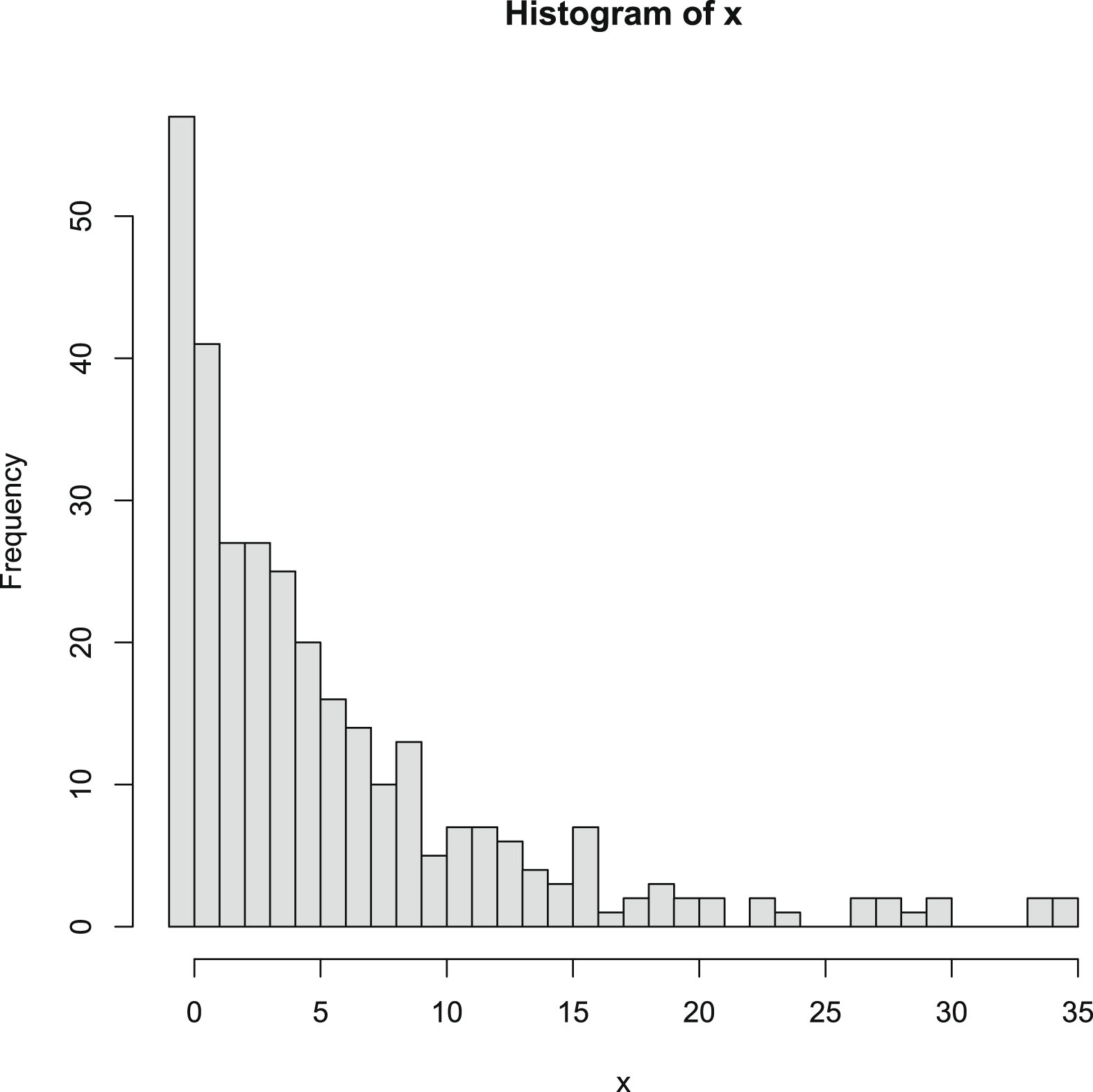
is depicted in figure 8.6. From the figure, we see that the data are right-skewed with a large variance.
FIG. 8.6 — P-G: The histogram of the sample  .
.
.
The estimators of the hyperparameters  and
and  , the goodness-of-fit of the model, the empirical Bayes estimators of the parameter of the Poisson distribution with a conjugate gamma prior (8.1) and the PESLs, and the mean and variance of the attendance data by the moment method and the MLE method are summarized in table 8.8. From the table, we observe the following facts.
and , the goodness-of-fit of the model, the empirical Bayes estimators of the parameter of the Poisson distribution with a conjugate gamma prior (8.1) and the PESLs, and the mean and variance of the attendance data by the moment method and the MLE method are summarized in table 8.8. From the table, we observe the following facts.
TAB. 8.8 — P-G: The estimators of the hyperparameters, the goodness-of-fit of the model, the empirical Bayes estimators of the parameter of the Poisson distribution with a conjugate gamma prior and the PESLs, and the mean and variance of the attendance data by the moment method and the MLE method.
| Moment method | MLE method | ||
| Estimators of the hyperparameters |  |
 |
 |
 |
 |
 |
|
| Goodness-of-fit of the model |  |
36 | 36 |
 |
313 | 313 | |
 |
31.379 | 30.702 | |
 |
33 | 33 | |
| p-value | 0.548 | 0.582 | |
| Empirical Bayes estimators and PESLs |  |
1.5994 | 1.5863 |
 |
2.4787 | 2.4683 | |
 |
0.2504 | 0.2530 | |
 |
0.3621 | 0.3668 | |
| Mean and variance of the attendance data |  |
5.968 | 5.968 |
 |
49.469 | 50.574 |
1. The sample size is  , which is divided into
  groups.
, which is divided into groups.
2. The degrees of freedom  , since two hyperparameters
  and
and  are estimated by the sample.
, since two hyperparameters and are estimated by the sample.
3. The p-value of the moment method is  , and thus the
  distribution with
  and
and  estimated by their moment estimators, fits the sample
  well. Similarly, the p-value of the MLE method is
  , and thus the
  distribution with
  and
and  estimated by their MLEs fits the sample
  well. Comparing the two methods, the
  value of the MLEs is smaller, and the p-value of the MLEs is larger, which means that the
  distribution with the hyperparameters
  and
and  estimated by the MLEs has a better fit to the sample
  than that estimated by the moment estimators.
, and thus the distribution with and estimated by their moment estimators, fits the sample well. Similarly, the p-value of the MLE method is , and thus the distribution with and estimated by their MLEs fits the sample well. Comparing the two methods, the value of the MLEs is smaller, and the p-value of the MLEs is larger, which means that the distribution with the hyperparameters and estimated by the MLEs has a better fit to the sample than that estimated by the moment estimators.
4. When the hyperparameters are estimated by the MLE method, we have

and

When the hyperparameters are estimated by the moment method, we observe a similar phenomenon for the Bayes estimators and the PESLs. Therefore, the two inequalities (8.6) and (8.9) are exemplified. Comparing the moment method and the MLE method, we see that the estimators of the hyperparameters, the Bayes estimators, the PESLs, and the mean and variance of the attendance data are very similar.
8.5 Conclusions and Discussions
For the hierarchical Poisson and gamma model (8.1), we first calculate the posterior distribution of  ,
,  , and the marginal pmf of
  ,
,  , in Theorem 8.1. We then calculate the Bayes estimators
  and
and  , and the PESLs
  and
and  , and they satisfy two inequalities (8.6) and (8.9). After that, the estimators of the hyperparameters of the model (8.1) by the moment method and their consistencies are summarized in Theorem 8.2. Moreover, the estimators of the hyperparameters of the model (8.1) by the MLE method and their consistencies are summarized in Theorem 8.3. Finally, the empirical Bayes estimators of the parameter of the model (8.1) under Stein’s loss function by the moment method and the MLE method are summarized in Theorem 8.4.
, , and the marginal pmf of , , in Theorem 8.1. We then calculate the Bayes estimators and , and the PESLs and , and they satisfy two inequalities (8.6) and (8.9). After that, the estimators of the hyperparameters of the model (8.1) by the moment method and their consistencies are summarized in Theorem 8.2. Moreover, the estimators of the hyperparameters of the model (8.1) by the MLE method and their consistencies are summarized in Theorem 8.3. Finally, the empirical Bayes estimators of the parameter of the model (8.1) under Stein’s loss function by the moment method and the MLE method are summarized in Theorem 8.4.
We carry out the numerical simulations for the hierarchical Poisson and gamma model (8.1) in the simulations section in four aspects. First, we have exemplified the two inequalities (8.6) and (8.9). Second, we have illustrated that the moment estimators and the MLEs are consistent estimators of the hyperparameters in table 8.4. Third, we have calculated the goodness-of-fit of the model (8.1) to the simulated data in table 8.5. Two cases of the goodness-of-fit have been considered. In the first case, the hyperparameters  and
and  are assumed to be known. In the second case, the hyperparameters
  and
and  are unknown, and this is also the case encountered in real applications. Finally, we have plotted the marginal pmfs of the model (8.1) for various hyperparameters.
and are assumed to be known. In the second case, the hyperparameters and are unknown, and this is also the case encountered in real applications. Finally, we have plotted the marginal pmfs of the model (8.1) for various hyperparameters.
In the real data example section, we exploit the attendance data on 314 high school juniors from two urban high schools in the file nb_data. The variable of interest is days absent, daysabs. The estimators of the hyperparameters, the goodness-of-fit of the model, the empirical Bayes estimators of the parameter of the Poisson distribution with a conjugate gamma prior and the PESLs, and the mean and variance of the attendance data by the moment method and the MLE method are summarized in table 8.8. Comparing the two methods, the  value of the MLEs is smaller, and the p-value of the MLEs is larger, which means that the
  distribution with the hyperparameters estimated by the MLEs has a better fit to the sample than that estimated by the moment estimators.
value of the MLEs is smaller, and the p-value of the MLEs is larger, which means that the distribution with the hyperparameters estimated by the MLEs has a better fit to the sample than that estimated by the moment estimators.
In empirical Bayes analysis, the hyperparameters are unknown, and the marginal distribution is used to estimate the hyperparameters from the observations. There are two common methods to estimate the hyperparameters by exploiting the marginal distribution: the moment method and the MLE method. In this chapter, we use the two methods to estimate the hyperparameters of the hierarchical Poisson and gamma model (8.1).
Exercise 4.32 (p. 196) of Casella and Berger (2002) and the particular part of Theorem 8.1 state that when  is a positive integer, the marginal distribution of the hierarchical Poisson and gamma model (8.1) is a negative binomial distribution. Therefore, the negative binomial data should have a good result of the goodness-of-fit of the model (8.1). In addition, the hierarchical Poisson and gamma model (8.1) is more general than the negative binomial distribution, as
  could be a general positive number in the model (8.1).
is a positive integer, the marginal distribution of the hierarchical Poisson and gamma model (8.1) is a negative binomial distribution. Therefore, the negative binomial data should have a good result of the goodness-of-fit of the model (8.1). In addition, the hierarchical Poisson and gamma model (8.1) is more general than the negative binomial distribution, as could be a general positive number in the model (8.1).
Inspired by the real data example, when the sample unconditional mean of the outcome variable is lower than its variance, then the Poisson model is not appropriate; however, the hierarchical Poisson and gamma model (8.1) should be adopted.
Comparing the two Bayes estimators  and
and  , we prefer the former one, not because it is larger or smaller than the latter one, but because Stein’s loss function is more appropriate than the squared error loss function for the positive parameter
  , as Stein’s loss function penalizes gross overestimation and gross underestimation equally for
  , while the squared error loss function does not.
and , we prefer the former one, not because it is larger or smaller than the latter one, but because Stein’s loss function is more appropriate than the squared error loss function for the positive parameter , as Stein’s loss function penalizes gross overestimation and gross underestimation equally for , while the squared error loss function does not.
Now we present some future work. One may consider extending the hierarchical Poisson and gamma model (8.1) to different types of non-conjugate priors for the parameter of the Poisson distribution (see Berger et al. (2015); Berger (1985, 2006) and the references therein). In these situations, one may not obtain analytical solutions, then one should be able to derive the estimators numerically.
Chapter 9 Several Common Loss Functions
In this chapter, we will introduce several common loss functions.
As discussed in Zhang et al. (2023), a good loss function  on
on  should have the following seven properties:
on should have the following seven properties:
(a)  for all
  ;
;
for all ;
(b)  ;
;
;
(c)  ;
;
;
(d)  ;
;
;
(e) convex in  ;
;
;
(f)  ;
;
;
(g)  for some
  .
.
for some .
Property (a) means that any action  of the parameter
  should incur a non-negative loss. Property (b) means that when
  , or
, or  , or
, or  correctly estimates
  , the loss is 0. Property (c) means that when
  , that is,
  is moving away from
  and tends to
  , it will incur an infinite loss. Property (d) means that when
  , that is,
  is moving away from
  and tends to
  , it will also incur an infinite loss. Properties (c) and (d) mean that the loss function will penalize gross overestimation and gross underestimation equally. Property (e) is useful in the proofs of some propositions of the minimaxity and admissibility of the Bayes estimator (see Robert (2007)). Property (f) implies that
  , that is, the loss incurred by an action
  near
near  (
( ) is very small compared to
  . Property (f) seems strange; however, it is satisfied by many loss functions. Property (g) means that
  and
and  for some
  tend to
  at the same rate, that is,

of the parameter should incur a non-negative loss. Property (b) means that when , or , or correctly estimates , the loss is 0. Property (c) means that when , that is, is moving away from and tends to , it will incur an infinite loss. Property (d) means that when , that is, is moving away from and tends to , it will also incur an infinite loss. Properties (c) and (d) mean that the loss function will penalize gross overestimation and gross underestimation equally. Property (e) is useful in the proofs of some propositions of the minimaxity and admissibility of the Bayes estimator (see Robert (2007)). Property (f) implies that , that is, the loss incurred by an action near () is very small compared to . Property (f) seems strange; however, it is satisfied by many loss functions. Property (g) means that and for some tend to at the same rate, that is,
And we say  and
and  are asymptotically equivalent. We also say that
  has balanced convergence rates or penalties for
  too large and
  too small. Property (g) may hold only when properties (c) and (d) hold.
and are asymptotically equivalent. We also say that has balanced convergence rates or penalties for too large and too small. Property (g) may hold only when properties (c) and (d) hold.
It is worth mentioning that all the loss functions in this chapter, except the two loss functions in section 9.3, satisfy properties (a)–(c). Moreover, all the loss functions satisfy

The rest of the chapter is organized as follows. In section 9.1, we will introduce two loss functions on  , the squared error loss function and the weighted squared error loss function. In section 9.2, we will introduce two loss functions on
  , Stein’s loss function and the power-power loss function. In section 9.3, we will introduce two loss functions on
  , the power-log loss function and Zhang’s loss function. In section 9.4, we will give three strings of inequalities among six Bayes estimators under six loss functions in sections 9.1–9.3. In section 9.5, we will introduce several other loss functions, which are meaningful on
  . In section 9.6, we will give a summary of the loss functions.
, the squared error loss function and the weighted squared error loss function. In section 9.2, we will introduce two loss functions on , Stein’s loss function and the power-power loss function. In section 9.3, we will introduce two loss functions on , the power-log loss function and Zhang’s loss function. In section 9.4, we will give three strings of inequalities among six Bayes estimators under six loss functions in sections 9.1–9.3. In section 9.5, we will introduce several other loss functions, which are meaningful on . In section 9.6, we will give a summary of the loss functions.
9.1 Two Loss Functions on Θ = (−∞, ∞)
9.1.1 Squared Error Loss Function
The squared error loss function in terms of  is given by
 (9.1)
where
(9.1)
where  and
and  . It is useful to point out that
  is used to guarantee that
  satisfies (c). Note that
  . The squared error loss function in terms of
  and
and  is given by
 (9.2)
where
(9.2)
where  .
.
is given by
(9.1)
and . It is useful to point out that is used to guarantee that satisfies (c). Note that . The squared error loss function in terms of and is given by
(9.2)
.
The squared error loss function in terms of  and the squared error loss function in terms of
  and
and  are plotted in figure 9.1. From the figure, we observe the following facts.
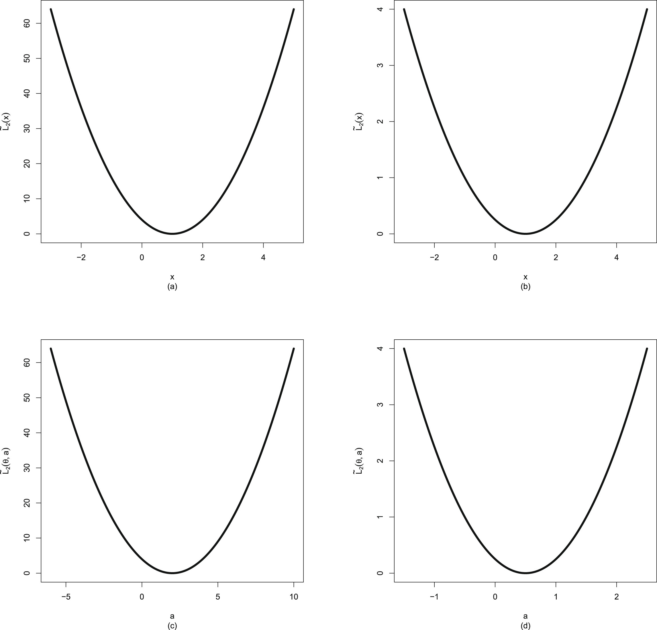
and the squared error loss function in terms of and are plotted in figure 9.1. From the figure, we observe the following facts.
1.  with
with  and
and  satisfies (a)–(f).
with and satisfies (a)–(f).
2. Plots (a) and (c) are the same, with the only difference being the  -axis ranges and labels, which are
  and
and  with a relation
  . Plots (b) and (d) are the same, with the only difference being the
  -axis ranges and labels, which are
  and
and  with a relation
  .
.
-axis ranges and labels, which are and with a relation . Plots (b) and (d) are the same, with the only difference being the -axis ranges and labels, which are and with a relation .
3. The ranges of  for plots (a) and (b) are
  . The range of
  for plot (c) is
  , as
, as  . The range of
  for plot (d) is
  , as
, as  .
.
for plots (a) and (b) are . The range of for plot (c) is , as . The range of for plot (d) is , as .
FIG. 9.1 — SCLF: The squared error loss function in terms of  and the squared error loss function in terms of
  and
and  . (a)
. (a)  with
with  . (b)
. (b)  with
with  . (c)
. (c)  with
with  . (d)
. (d)  with
with  .
.
and the squared error loss function in terms of and . (a) with . (b) with . (c) with . (d) with .
9.1.2 Weighted Squared Error Loss Function
The weighted squared error loss function in terms of  is given by
 (9.3)
where
(9.3)
where  . Note that
  . The weighted squared error loss function in terms of
  and
and  is given by
 (9.4)
where
(9.4)
where  and
and  . Note that the weighted squared error loss function
  has weight
  .
.
is given by
(9.3)
. Note that . The weighted squared error loss function in terms of and is given by
(9.4)
and . Note that the weighted squared error loss function has weight .
The weighted squared error loss function in terms of  and the weighted squared error loss function in terms of
  and
and  are plotted in figure 9.2. From the figure, we observe the following facts.
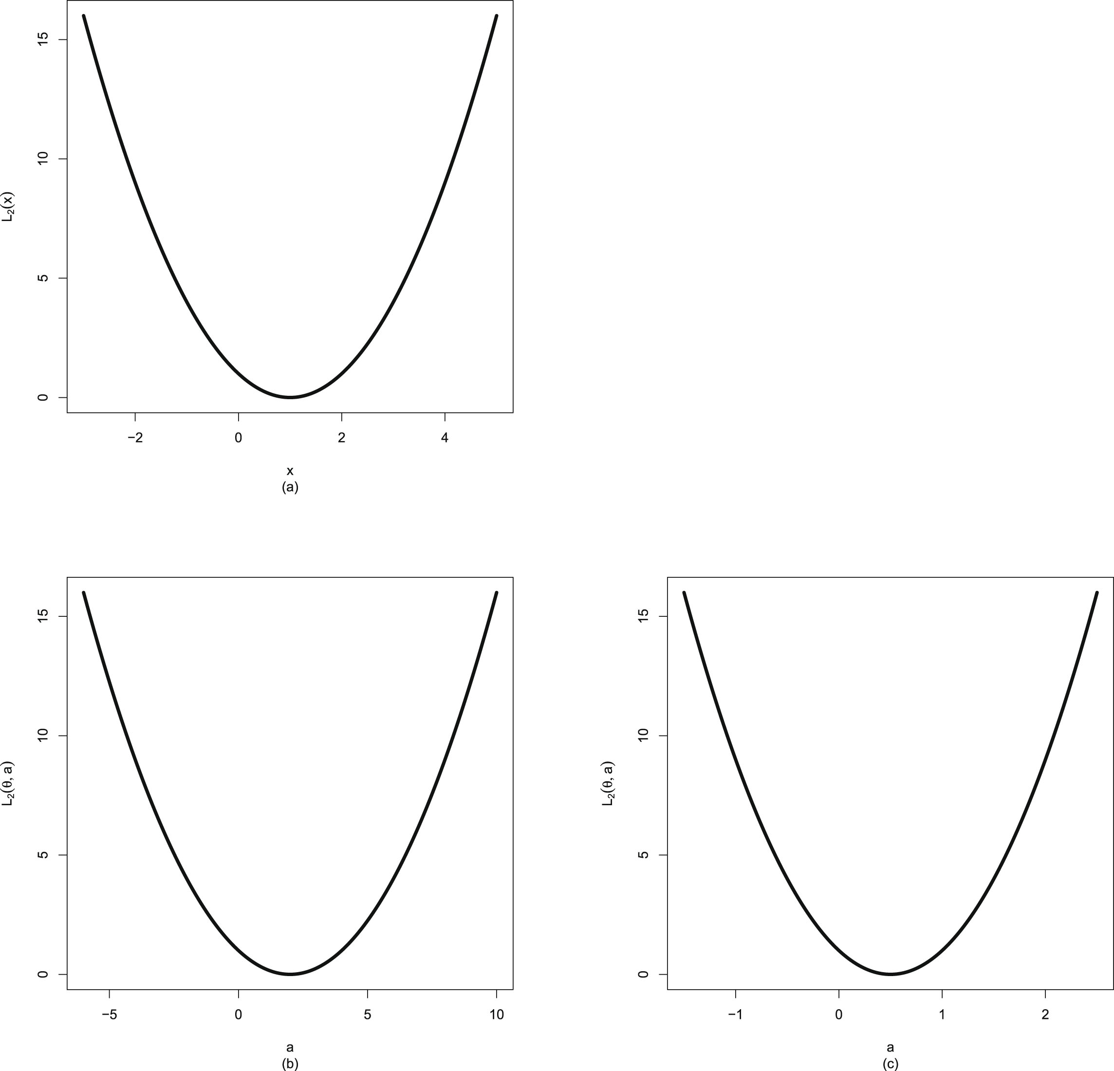
and the weighted squared error loss function in terms of and are plotted in figure 9.2. From the figure, we observe the following facts.
1.  satisfies (a)–(f).
satisfies (a)–(f).
2. Plots (a) and (b) ((a) and (c)) are the same, with the only differences being the  -axis ranges and labels, which are
  and
and  with a relation
  .
.
-axis ranges and labels, which are and with a relation .
3. The range of  for plot (a) is
  . The range of
  for plot (b) is
  , as
, as  . The range of
  for plot (c) is
  , as
, as  .
.
for plot (a) is . The range of for plot (b) is , as . The range of for plot (c) is , as .
FIG. 9.2 — SCLF: The weighted squared error loss function in terms of  and the weighted squared error loss function in terms of
  and
and  . (a)
. (a)  . (b)
. (b)  with
with  . (c)
. (c)  with
with  .
.
and the weighted squared error loss function in terms of and . (a) . (b) with . (c) with .
9.2 Two Loss Functions on Θ = (0, ∞)
9.2.1 Stein’s Loss Function
Stein’s loss function in terms of  is given by
 (9.5)
where
(9.5)
where  . Note that
  . Stein’s loss function in terms of
  and
and  is given by
 (9.6)
where
(9.6)
where  . Stein’s loss function penalizes gross overestimation and gross underestimation equally, that is, an action a will incur an infinite loss when it tends to 0 or ∞. Therefore, Stein’s loss function is a good loss function and it is recommended to use for the positive parameter space by many authors (see for instance Li et al. (2025); Shi et al. (2025); Zhang (2025); Sun et al. (2024); Zhang et al. (2024); Sun et al. (2021); Xie et al. (2018); Zhang et al. (2018, 2019b); Zhang (2017); Bobotas and Kourouklis (2010); Petropoulos and Kourouklis (2005); Oono and Shinozaki (2006); Parsian and Nematollahi (1996); Brown (1968, 1990); James and Stein (1961)).
is given by
(9.5)
. Note that . Stein’s loss function in terms of and is given by
(9.6)
. Stein’s loss function penalizes gross overestimation and gross underestimation equally, that is, an action a will incur an infinite loss when it tends to 0 or ∞. Therefore, Stein’s loss function is a good loss function and it is recommended to use for the positive parameter space by many authors (see for instance Li et al. (2025); Shi et al. (2025); Zhang (2025); Sun et al. (2024); Zhang et al. (2024); Sun et al. (2021); Xie et al. (2018); Zhang et al. (2018, 2019b); Zhang (2017); Bobotas and Kourouklis (2010); Petropoulos and Kourouklis (2005); Oono and Shinozaki (2006); Parsian and Nematollahi (1996); Brown (1968, 1990); James and Stein (1961)).
Stein’s loss function in terms of  and Stein’s loss function in terms of
  and
and  are plotted in figure 9.3. From the figure, we observe the following facts.
and Stein’s loss function in terms of and are plotted in figure 9.3. From the figure, we observe the following facts.
1.  satisfies (a)–(f).
satisfies (a)–(f).
2. Plots (a) and (b) ((a) and (c)) are the same, with the only differences being the  -axis ranges and labels, which are
  and
and  with a relation
  .
.
-axis ranges and labels, which are and with a relation .
3. The range of  for plot (a) is
  . The range of
  for plot (b) is
  , as
, as  . The range of
  for plot (c) is
  , as
, as  .
.
for plot (a) is . The range of for plot (b) is , as . The range of for plot (c) is , as .
9.2.2 Power-Power Loss Function
The main reference of this subsection is Zhang et al. (2023).
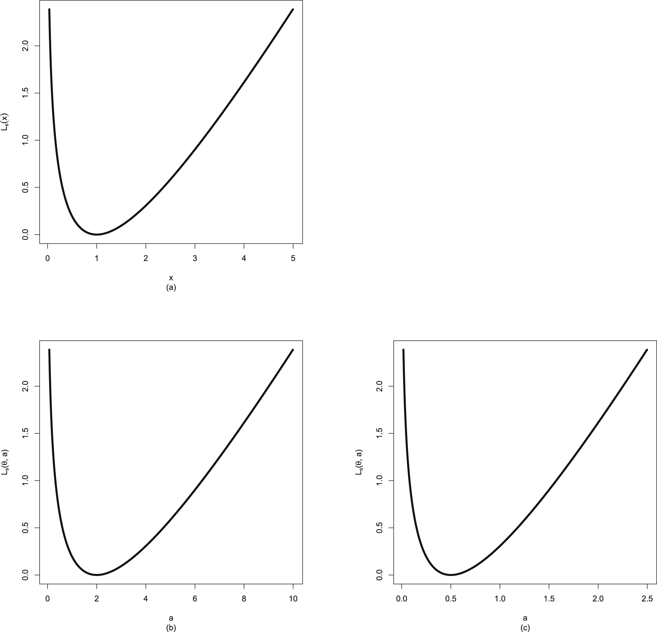
FIG. 9.3 — SCLF: Stein’s loss function in terms of  and Stein’s loss function in terms of
  and
and  . (a)
. (a)  . (b)
. (b)  with
with  . (c)
. (c)  with
with  .
.
and Stein’s loss function in terms of and . (a) . (b) with . (c) with .
Many authors have used the (weighted) squared error loss function for the problem of estimating the variance,  , based on a random sample from a normal distribution with mean
  unknown (see, for instance, Maatta and Casella (1990); Stein (1964)). As pointed out by Casella and Berger (2002), the (weighted) squared error loss function penalizes equally for overestimation and underestimation, which is fine in the location case with
  . In the positive parameter case with
  where 0 is a natural lower bound and the estimation problem is not symmetric, we should not choose the (weighted) squared error loss function, but choose a loss function which penalizes gross overestimation and gross underestimation equally, that is, an action
  will incur an infinite loss when it tends to 0 or
  . Stein’s loss function
  has this property, and thus it is recommended to use for the positive parameter space
  by many authors. However,
 that is,
  tends to
  much faster than
  for any
  , which means that
  has unbalanced convergence rates or penalties for
  too large and
  too small. Zhang et al. (2023) propose the power-power loss function
  which has the property that
  and
and  tend to
  at the same rate, that is,
  has balanced convergence rates or penalties for
  too large and
  too small. Therefore, the power-power loss function
  is recommended to use for the positive parameter space
  .
.
, based on a random sample from a normal distribution with mean unknown (see, for instance, Maatta and Casella (1990); Stein (1964)). As pointed out by Casella and Berger (2002), the (weighted) squared error loss function penalizes equally for overestimation and underestimation, which is fine in the location case with . In the positive parameter case with where 0 is a natural lower bound and the estimation problem is not symmetric, we should not choose the (weighted) squared error loss function, but choose a loss function which penalizes gross overestimation and gross underestimation equally, that is, an action will incur an infinite loss when it tends to 0 or . Stein’s loss function has this property, and thus it is recommended to use for the positive parameter space by many authors. However,
tends to much faster than for any , which means that has unbalanced convergence rates or penalties for too large and too small. Zhang et al. (2023) propose the power-power loss function which has the property that and tend to at the same rate, that is, has balanced convergence rates or penalties for too large and too small. Therefore, the power-power loss function is recommended to use for the positive parameter space .
The power-power loss function (see Zhang et al. (2023)) in terms of  is given by
 (9.7)
where
(9.7)
where  . Note that
  . The power-power loss function in terms of
  and
and  is given by
 (9.8)
where
(9.8)
where  .
.
is given by
(9.7)
. Note that . The power-power loss function in terms of and is given by
(9.8)
.
The power-power loss function  has all the seven properties (a)-(g). In particular, the power-power loss function penalizes gross overestimation and gross underestimation equally, that is, an action
  will incur an infinite loss when it tends to 0 or
  .
.
has all the seven properties (a)-(g). In particular, the power-power loss function penalizes gross overestimation and gross underestimation equally, that is, an action will incur an infinite loss when it tends to 0 or .
The power-power loss function in terms of  and the power-power loss function in terms of
  and
and  are plotted in figure 9.4. From the figure, we observe the following facts.
and the power-power loss function in terms of and are plotted in figure 9.4. From the figure, we observe the following facts.
1.  satisfies (a)–(g) with
  .
.
satisfies (a)–(g) with .
2. From plot (a), we see that the  values of the markers are given by

values of the markers are given by
We see that

Therefore,  satisfies (g) with
  .
.
satisfies (g) with .
3. Plots (a) and (b) ((a) and (c)) are the same, with the only differences being the  -axis ranges and labels, which are
  and
and  with a relation
  .
.
-axis ranges and labels, which are and with a relation .
4. The range of  for plot (a) is
  . The range of
  for plot (b) is
  , as
, as  . The range of
  for plot (c) is
  , as
, as  .
.
for plot (a) is . The range of for plot (b) is , as . The range of for plot (c) is , as .
In Zhang et al. (2023), they calculate the Bayes estimator  of the parameter
  under the power-power loss function
  , the Posterior Expected Power-power Loss (PEPL) at
  ,
,  , and the Integrated Risk under Power-power Loss (IRPL) at
  ,
,  , which is also the Bayes Risk under Power-power Loss (BRPL). They also calculate three other Bayes estimators
  ,
,  , and
, and  , and each Bayes estimator minimizes some posterior expected loss function. It is interesting to note that the four Bayes estimators satisfy a string of inequalities. After that, they analytically calculate the Bayes estimator
  , the PEPL at
  , and the BRPL under a hierarchical normal and normal-inverse-gamma model.
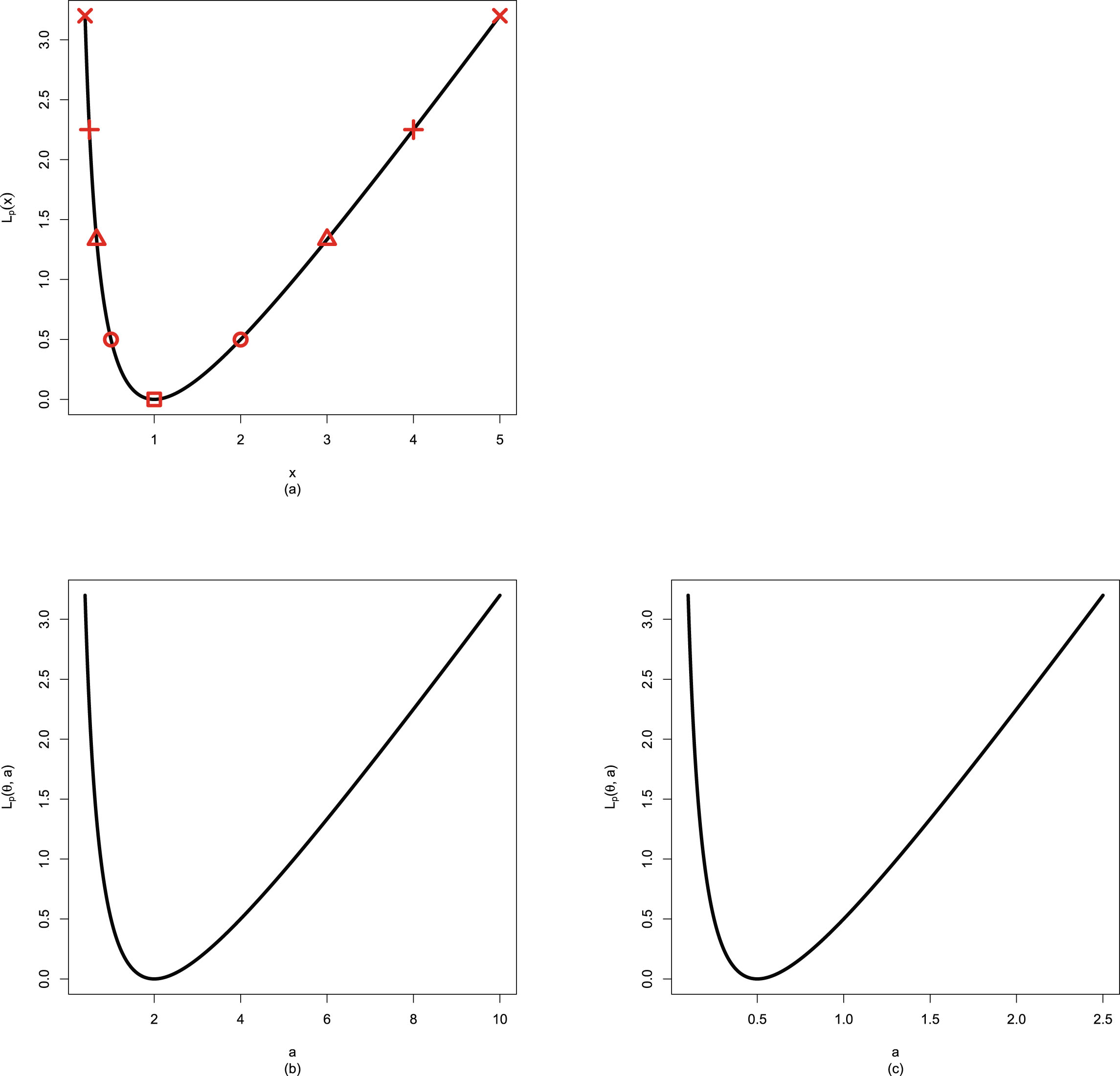
of the parameter under the power-power loss function , the Posterior Expected Power-power Loss (PEPL) at , , and the Integrated Risk under Power-power Loss (IRPL) at , , which is also the Bayes Risk under Power-power Loss (BRPL). They also calculate three other Bayes estimators , , and , and each Bayes estimator minimizes some posterior expected loss function. It is interesting to note that the four Bayes estimators satisfy a string of inequalities. After that, they analytically calculate the Bayes estimator , the PEPL at , and the BRPL under a hierarchical normal and normal-inverse-gamma model.
FIG. 9.4 — SCLF: The power-power loss function in terms of  and the power-power loss function in terms of
  and
and  . (a)
. (a)  . (b)
. (b)  with
with  . (c)
. (c)  with
with  .
.
and the power-power loss function in terms of and . (a) . (b) with . (c) with .
9.3 Two Loss Functions on Θ = (0, 1)
9.3.1 Power-Log Loss Function
The main reference of this subsection is Zhang et al. (2017).
The (weighted) squared error loss function has been used by many authors for the problem of estimating the variance,  , based on a random sample from a normal distribution with unknown mean
  (see, for example Maatta and Casella (1990); Stein (1964)). As pointed out by Casella and Berger (2002), the (weighted) squared error loss function penalizes overestimation and underestimation equally, which is fine for the unrestricted parameter space
  . In the positive parameter space
  where 0 is a natural lower bound and the estimation problem is not symmetric, we should not select the (weighted) squared error loss function, but select a loss function which penalizes gross overestimation and gross underestimation equally, that is, an action
  will incur an infinite loss when it tends to 0 or
  . Stein’s loss function has this property, and thus it is recommended to use it for the positive parameter space
  by many authors. Similarly, for the restricted parameter space
  , where 0 and 1 are two natural bounds and the estimation problem is not symmetric, we should not choose the (weighted) squared error loss function, but choose a loss function which penalizes gross overestimation and gross underestimation equally, that is, an action
  will incur an infinite loss when it tends to 0 or 1. Note that Stein’s loss function is also not appropriate in this case. Zhang et al. (2017) list 6 properties summarized in table 9.3 for a good loss function on
  . After that, they propose the power-log loss function plotted in figure 9.5 on
  , which satisfies all the 6 properties listed in table 9.1. In particular, the power-log loss function penalizes gross overestimation and gross underestimation equally, is convex in
  or
or  , and attains its global minimum at
  or
or  . Therefore, the power-log loss function is recommended to use for
  . Finally, they remark that the power-log loss function on
  is an analog of the power-log loss function on
  , which is the popular Stein’s loss function.
, based on a random sample from a normal distribution with unknown mean (see, for example Maatta and Casella (1990); Stein (1964)). As pointed out by Casella and Berger (2002), the (weighted) squared error loss function penalizes overestimation and underestimation equally, which is fine for the unrestricted parameter space . In the positive parameter space where 0 is a natural lower bound and the estimation problem is not symmetric, we should not select the (weighted) squared error loss function, but select a loss function which penalizes gross overestimation and gross underestimation equally, that is, an action will incur an infinite loss when it tends to 0 or . Stein’s loss function has this property, and thus it is recommended to use it for the positive parameter space by many authors. Similarly, for the restricted parameter space , where 0 and 1 are two natural bounds and the estimation problem is not symmetric, we should not choose the (weighted) squared error loss function, but choose a loss function which penalizes gross overestimation and gross underestimation equally, that is, an action will incur an infinite loss when it tends to 0 or 1. Note that Stein’s loss function is also not appropriate in this case. Zhang et al. (2017) list 6 properties summarized in table 9.3 for a good loss function on . After that, they propose the power-log loss function plotted in figure 9.5 on , which satisfies all the 6 properties listed in table 9.1. In particular, the power-log loss function penalizes gross overestimation and gross underestimation equally, is convex in or , and attains its global minimum at or . Therefore, the power-log loss function is recommended to use for . Finally, they remark that the power-log loss function on is an analog of the power-log loss function on , which is the popular Stein’s loss function.
TAB. 9.1 — SCLF: The 6 properties of a good loss function on  .
.  is fixed.
. is fixed.
| Properties |  |
 |
| (a) |  for all for all  |
 for all for all  |
| (b) |  |
 |
| (c) |  |
 |
| (d) |  |
 |
| (e) | convex in  for all for all  |
convex in  for all for all  |
| (f) |  |
 |
A natural model with the restricted parameter space  is the beta-binomial mode, which has been investigated extensively. For instance, Prentice (1986) extended the beta-binomial distribution to allow negative correlations among binary variates within an experimental unit. Lee and Sabavala (1987) proposed a Bayesian approach with a conjugate-type beta family of priors for suitably transformed parameters in the beta-binomial, and demonstrated the simulations for a special case of two trials. Lee and Lio (1999) extended the study of Lee and Sabavala (1987) by a numerical double integration, which can be used for the case of general trials. Ali-Mousa (1988) studied the risk of the linear empirical Bayes estimate of the binomial parameter
  . Rosner (1989) proposed a compound beta-binomial distribution that generalized the beta-binomial distribution to more than one level of nesting. Wypij and Santner (1990) studied the problem of confidence interval estimation of the common marginal probability of success for correlated binary observations, focusing on the beta-binomial model. Srivastava and Wu (1993) introduced the beta-binomial model as a Markov chain. They have shown that, locally, the moment estimator for the mean is efficient up to the second order of the extra-binomial variation. Aerts and Claeskens (1997) illustrated how the local likelihood estimation procedure can be implemented for fitting a dose-response curve based on the beta-binomial model. Karunamuni and Prasad (2003) investigated empirical Bayes sequential procedures for estimates of binomial probabilities. Hunt et al. (2009) exploited the beta-binomial distribution for estimating the number of false rejections in microarray gene expression studies. Moreover, an estimator of the beta-binomial false discovery rate is then derived. Kolossiatis et al. (2011) modeled overdispersion with the multivariate normalized tempered stable distribution. The univariate version of the distribution was used as a mixing distribution for the success probability of a binomial distribution to define an alternative to the beta-binomial distribution. Hout et al. (2013) presented the binomial and the beta-binomial distributions as alternatives to the normal distribution for the sum score of a cognitive test. Larson et al. (2015) took into account novel application of beta-binomial models to assess x chromosome inactivation patterns in RNA-seq expression of ovarian tumors. Chen et al. (2016) investigated meta-analysis of studies with bivariate binary outcomes by using a marginal beta-binomial model approach. Tak and Morris (2017) researched data-dependent posterior propriety of a Bayesian beta-binomial-logit model. Luo and Paul (2018) considered estimation for a zero-inflated beta-binomial regression model with missing response data. Najera-Zuloaga et al. (2019) proposed a beta-binomial mixed-effects model approach for analysing longitudinal discrete and bounded outcomes. Zhang et al. (2020) considered the Bayes rule of the parameter in
  under Zhang’s loss function with an application to the beta-binomial model. Palm et al. (2021) studied signal detection and inference based on the beta-binomial autoregressive moving average model. Felsch et al. (2022) researched the performance of several types of beta-binomial models in comparison to standard approaches for meta-analyses with very few studies. Cmiel et al. (2024) studied generalised score distribution by using underdispersed continuation of the beta-binomial distribution.
is the beta-binomial mode, which has been investigated extensively. For instance, Prentice (1986) extended the beta-binomial distribution to allow negative correlations among binary variates within an experimental unit. Lee and Sabavala (1987) proposed a Bayesian approach with a conjugate-type beta family of priors for suitably transformed parameters in the beta-binomial, and demonstrated the simulations for a special case of two trials. Lee and Lio (1999) extended the study of Lee and Sabavala (1987) by a numerical double integration, which can be used for the case of general trials. Ali-Mousa (1988) studied the risk of the linear empirical Bayes estimate of the binomial parameter . Rosner (1989) proposed a compound beta-binomial distribution that generalized the beta-binomial distribution to more than one level of nesting. Wypij and Santner (1990) studied the problem of confidence interval estimation of the common marginal probability of success for correlated binary observations, focusing on the beta-binomial model. Srivastava and Wu (1993) introduced the beta-binomial model as a Markov chain. They have shown that, locally, the moment estimator for the mean is efficient up to the second order of the extra-binomial variation. Aerts and Claeskens (1997) illustrated how the local likelihood estimation procedure can be implemented for fitting a dose-response curve based on the beta-binomial model. Karunamuni and Prasad (2003) investigated empirical Bayes sequential procedures for estimates of binomial probabilities. Hunt et al. (2009) exploited the beta-binomial distribution for estimating the number of false rejections in microarray gene expression studies. Moreover, an estimator of the beta-binomial false discovery rate is then derived. Kolossiatis et al. (2011) modeled overdispersion with the multivariate normalized tempered stable distribution. The univariate version of the distribution was used as a mixing distribution for the success probability of a binomial distribution to define an alternative to the beta-binomial distribution. Hout et al. (2013) presented the binomial and the beta-binomial distributions as alternatives to the normal distribution for the sum score of a cognitive test. Larson et al. (2015) took into account novel application of beta-binomial models to assess x chromosome inactivation patterns in RNA-seq expression of ovarian tumors. Chen et al. (2016) investigated meta-analysis of studies with bivariate binary outcomes by using a marginal beta-binomial model approach. Tak and Morris (2017) researched data-dependent posterior propriety of a Bayesian beta-binomial-logit model. Luo and Paul (2018) considered estimation for a zero-inflated beta-binomial regression model with missing response data. Najera-Zuloaga et al. (2019) proposed a beta-binomial mixed-effects model approach for analysing longitudinal discrete and bounded outcomes. Zhang et al. (2020) considered the Bayes rule of the parameter in under Zhang’s loss function with an application to the beta-binomial model. Palm et al. (2021) studied signal detection and inference based on the beta-binomial autoregressive moving average model. Felsch et al. (2022) researched the performance of several types of beta-binomial models in comparison to standard approaches for meta-analyses with very few studies. Cmiel et al. (2024) studied generalised score distribution by using underdispersed continuation of the beta-binomial distribution.
A good loss function  on
on 
on
A good loss function  on
on  should have the 6 properties summarized in table 9.1. In the table, we observe the following facts.
on should have the 6 properties summarized in table 9.1. In the table, we observe the following facts.
1. Property (a) means that any action  of the parameter
  should incur a non-negative loss.
of the parameter should incur a non-negative loss.
2. Property (b) means that when  , or
, or  , that is,
  correctly estimates
  , the loss is 0.
, or , that is, correctly estimates , the loss is 0.
3. Property (c) means that when  , that is,
  is moving away from
  and tends to
  , it will incur an infinite loss.
, that is, is moving away from and tends to , it will incur an infinite loss.
4. Property (d) means that when  , that is,
  is moving away from
  and tends to
  , it will also incur an infinite loss.
, that is, is moving away from and tends to , it will also incur an infinite loss.
5. Properties (c) and (d) mean that the loss function will penalize gross overestimation and gross underestimation equally.
6. Property (e) is useful in the proofs of some propositions of the minimaxity and the admissibility of the Bayes estimator (see Robert (2007)).
7. Property (f) means that 1 and  are the local extrema of
  and
and  respectively. Property (f) also implies that
  , that is, the loss incurred by an action
  near
near  (
( ) is very small compared to
  .
.
are the local extrema of and respectively. Property (f) also implies that , that is, the loss incurred by an action near () is very small compared to .
Now let us give the analytical forms of the power-log loss function. Let

Define
 (9.9)
(9.9)
(9.9)
Thus
 (9.10)
(9.10)
Note that  is the power-log loss function in terms of
  and
and  is the power-log loss function in terms of
  and
and  . It is easy to check that the power-log loss functions
  and
and  satisfy all 6 properties listed in table 9.1. Therefore, the power-log loss function is a good loss function on
  . We remark that the power-log loss function on
  is an analog of the power-log loss function on
  , which is the popular Stein’s loss function given by (9.6).
is the power-log loss function in terms of and is the power-log loss function in terms of and . It is easy to check that the power-log loss functions and satisfy all 6 properties listed in table 9.1. Therefore, the power-log loss function is a good loss function on . We remark that the power-log loss function on is an analog of the power-log loss function on , which is the popular Stein’s loss function given by (9.6).
Figure 9.5 plots the power-log loss functions  and
and  . The two curves coincide in the two plots, with the only difference being the
  -axis ranges and labels, which are
  and
and  with a relation
  . The 6 properties listed in table 9.1 of
  and
and  are easily seen in the figure.
and . The two curves coincide in the two plots, with the only difference being the -axis ranges and labels, which are and with a relation . The 6 properties listed in table 9.1 of and are easily seen in the figure.
In Zhang et al. (2017), they calculate the Bayes estimator  of the parameter
  under the power-log loss function, the Posterior Expected Power-Log Loss (PEPLL) at
  ,
,  , and the Integrated Risk under the Power-Log Loss (IRPLL) at
  ,
,  , which is also the Bayes Risk under the Power-Log Loss (BRPLL). They also calculate the usual Bayes estimator
  . It is interesting to note that
  whose proof exploits the Covariance Inequality. After that, they analytically calculate
  and
and  , the PEPLL at
  and
and  under a beta-binomial model.
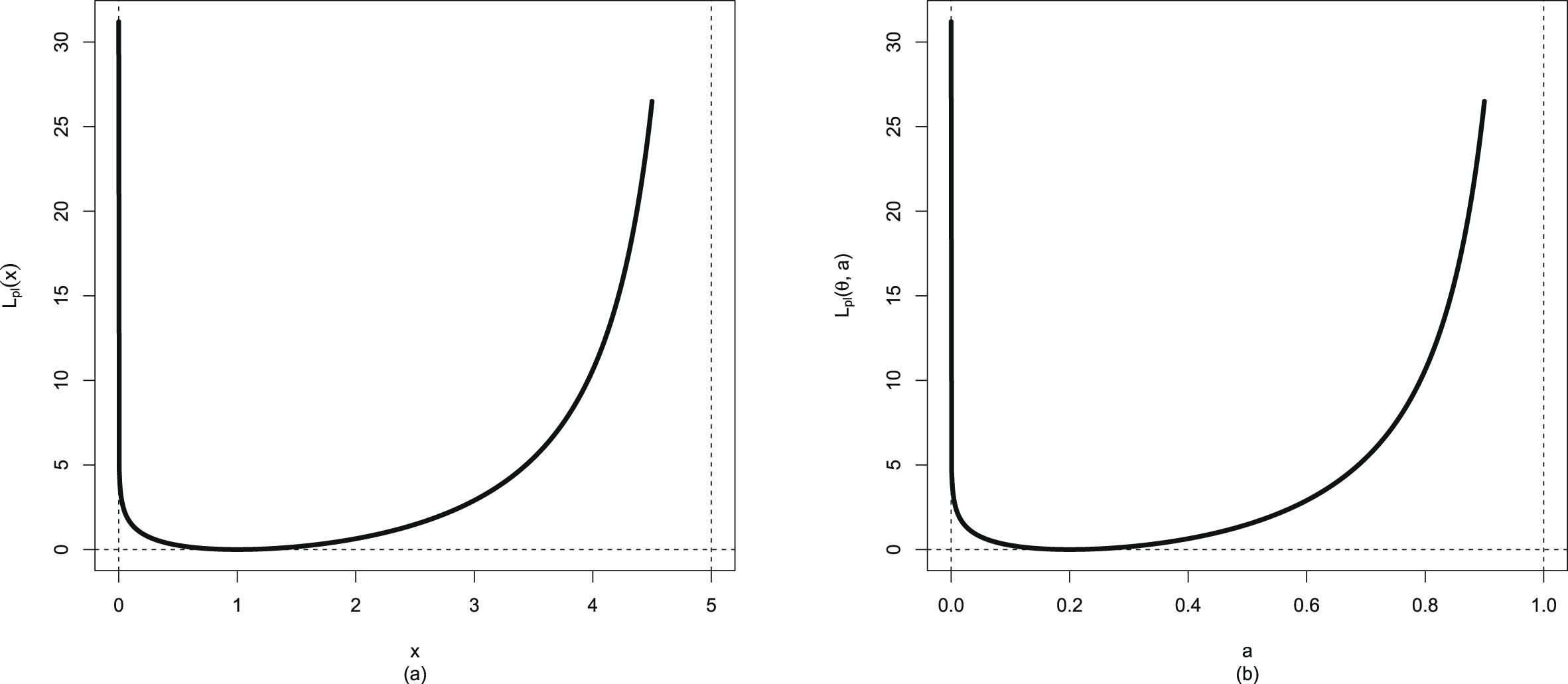
of the parameter under the power-log loss function, the Posterior Expected Power-Log Loss (PEPLL) at , , and the Integrated Risk under the Power-Log Loss (IRPLL) at , , which is also the Bayes Risk under the Power-Log Loss (BRPLL). They also calculate the usual Bayes estimator . It is interesting to note that whose proof exploits the Covariance Inequality. After that, they analytically calculate and , the PEPLL at and under a beta-binomial model.
FIG. 9.5 — SCLF: The power-log loss function in terms of  and the power-log loss function in terms of
  and
and  .
.  in both plots. (a)
  for
for  . (b)
. (b)  for
for  .
.
and the power-log loss function in terms of and . in both plots. (a) for . (b) for .
9.3.2 Zhang’s Loss Function
The main reference of this subsection is Zhang et al. (2020).
For the restricted parameter space  , where 0 and 1 are two natural bounds and the estimation problem is not symmetric, we should not choose the (weighted) squared error loss function, but choose a loss function which penalizes gross overestimation and gross underestimation equally, that is, an action
  will incur an infinite loss when it tends to 0 or 1. Note that Stein’s loss function is also not appropriate in this case. Zhang et al. (2017) propose the power-log loss function, which has this property with an application to the beta-binomial model. They propose 6 properties for a good loss function on
  . In particular, the power-log loss function penalizes gross overestimation and gross underestimation equally, is convex in its argument, and attains its global minimum at the true unknown parameter. In addition to the 6 properties, Zhang et al. (2020) propose the 7th property (balanced convergence rates or penalties for the argument too large and too small) for a good loss function on
  . The 7 properties for a good loss function on
  are summarized in table 9.2. After that, they propose Zhang’s loss function plotted in figure 9.6 on
  , which satisfies all the 7 properties listed in table 9.2. Therefore, Zhang’s loss function is recommended for use for
  .
.
, where 0 and 1 are two natural bounds and the estimation problem is not symmetric, we should not choose the (weighted) squared error loss function, but choose a loss function which penalizes gross overestimation and gross underestimation equally, that is, an action will incur an infinite loss when it tends to 0 or 1. Note that Stein’s loss function is also not appropriate in this case. Zhang et al. (2017) propose the power-log loss function, which has this property with an application to the beta-binomial model. They propose 6 properties for a good loss function on . In particular, the power-log loss function penalizes gross overestimation and gross underestimation equally, is convex in its argument, and attains its global minimum at the true unknown parameter. In addition to the 6 properties, Zhang et al. (2020) propose the 7th property (balanced convergence rates or penalties for the argument too large and too small) for a good loss function on . The 7 properties for a good loss function on are summarized in table 9.2. After that, they propose Zhang’s loss function plotted in figure 9.6 on , which satisfies all the 7 properties listed in table 9.2. Therefore, Zhang’s loss function is recommended for use for .
A natural model with the restricted parameter space  is the beta-binomial model. See Cmiel et al. (2024); Felsch et al. (2022); Palm et al. (2021); Zhang et al. (2020); Najera-Zuloaga et al. (2019); Luo and Paul (2018); Tak and Morris (2017); Zhang et al. (2017); Chen et al. (2016); Larson et al. (2015); Hout et al. (2013); Singh et al. (2013); Kolossiatis et al. (2011); Hunt et al. (2009); Karunamuni and Prasad (2003); Lee and Lio (1999); Aerts and Claeskens (1997); Srivastava and Wu (1993); Wypij and Santner (1990); Rosner (1989); Ali-Mousa (1988); Lee and Sabavala (1987); Prentice, (1986).
is the beta-binomial model. See Cmiel et al. (2024); Felsch et al. (2022); Palm et al. (2021); Zhang et al. (2020); Najera-Zuloaga et al. (2019); Luo and Paul (2018); Tak and Morris (2017); Zhang et al. (2017); Chen et al. (2016); Larson et al. (2015); Hout et al. (2013); Singh et al. (2013); Kolossiatis et al. (2011); Hunt et al. (2009); Karunamuni and Prasad (2003); Lee and Lio (1999); Aerts and Claeskens (1997); Srivastava and Wu (1993); Wypij and Santner (1990); Rosner (1989); Ali-Mousa (1988); Lee and Sabavala (1987); Prentice, (1986).
The 7 properties for a good loss function on  are summarized in table 9.2. The explanations of the first 6 properties in table 9.2 can be found in Zhang et al. (2017) or subsection 9.3.1 in this book. In table 9.2, property (g) means that
  and
and  ,
,  and
and  tend to
  at the same rate, that is,

are summarized in table 9.2. The explanations of the first 6 properties in table 9.2 can be found in Zhang et al. (2017) or subsection 9.3.1 in this book. In table 9.2, property (g) means that and , and tend to at the same rate, that is,
And we say  and
and  ,
,  and
and  are asymptotically equivalent. We also say that
  (
( ) has balanced convergence rates or penalties for
  (
( ) too large and too small. Note that
 and
and

and , and are asymptotically equivalent. We also say that () has balanced convergence rates or penalties for () too large and too small. Note that
That is,  and
and  at the same order
  . Similarly,
  and
and  at the same order
  . Property (g) may hold only when properties (c) and (d) hold.
and at the same order . Similarly, and at the same order . Property (g) may hold only when properties (c) and (d) hold.
TAB. 9.2 — SCLF: The 7 properties of a good loss function on  .
.  is fixed.
. is fixed.
| Properties |  |
 |
| (a) |  for all for all  |
 for all for all  |
| (b) |  |
 |
| (c) |  |
 |
| (d) |  |
 |
| (e) | convex in  for all for all  |
convex in  for all for all  |
| (f) |  |
 |
| (g) |  |
 |
Now let us give the analytical forms of Zhang’s loss function. Let

Let
 (9.11)
(9.11)
Thus
 (9.12)
(9.12)
Note that  is Zhang’s loss function in terms of
  and
and  is Zhang’s loss function in terms of
  and
and  . It is easy to check that Zhang’s loss function
  and
and  satisfy all the 7 properties listed in table 9.2. The check can be found in the supplement of Zhang et al. (2020). Therefore, Zhang’s loss function is a good loss function on
  .
.
is Zhang’s loss function in terms of and is Zhang’s loss function in terms of and . It is easy to check that Zhang’s loss function and satisfy all the 7 properties listed in table 9.2. The check can be found in the supplement of Zhang et al. (2020). Therefore, Zhang’s loss function is a good loss function on .
Figure 9.6 plots Zhang’s loss functions  and
and  . The two curves coincide in the two plots, with the only difference being the
  -axis ranges and labels, which are
  and
and  with a relation
  . The first 6 properties of
  and
and  are easily seen in the figure. Property (g) means that when
  is large,
 and
and

and . The two curves coincide in the two plots, with the only difference being the -axis ranges and labels, which are and with a relation . The first 6 properties of and are easily seen in the figure. Property (g) means that when is large,
We place the same markers on
 for
for  in the left plot of the figure. Similarly, we place the same markers on
 for
for  in the right plot of the figure. We see from both plots that the loss functions
  and
and  have balanced convergence rates or penalties for
  and
and  large and small, which means that property (g) holds.
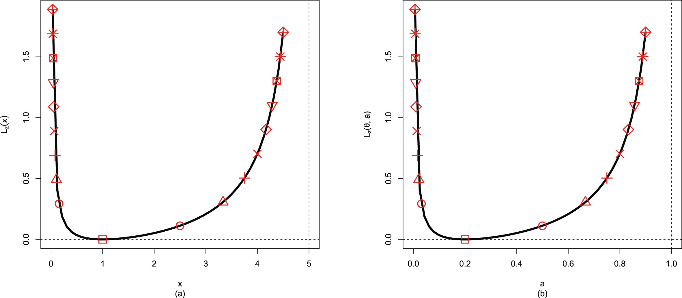
in the left plot of the figure. Similarly, we place the same markers on
in the right plot of the figure. We see from both plots that the loss functions and have balanced convergence rates or penalties for and large and small, which means that property (g) holds.
FIG. 9.6 — SCLF: Zhang’s loss function in terms of  and Zhang’s loss function in terms of
  and
and  .
.  in both plots. (a)
  for
for  . (b)
. (b)  for
for  .
.
and Zhang’s loss function in terms of and . in both plots. (a) for . (b) for .
9.4 Three Strings of Inequalities among Six Bayes Estimators
The main reference of this section is Zhang et al. (2018).
There are four basic elements in Bayesian decision theory: The data, the model, the prior, and the loss function. A Bayes point estimator minimizes some posterior expected loss function. In this section, we confine our interests to six loss functions: The weighted squared error loss function (Robert (2007) p. 78), the squared error loss function (well known), Stein’s loss function (Li et al. (2025); Shi et al. (2025); Zhang (2025); Sun et al. (2024); Zhang et al. (2024); Sun et al. (2021); Zhang et al. (2018, 2019b); Xie et al. (2018); Zhang (2017); Bobotas and Kourouklis (2010); Ye and Wang (2009); Oono and Shinozaki (2006); Petropoulos and Kourouklis (2005); Parsian and Nematollahi (1996); Brown (1990, 1968); James and Stein (1961)), the power-power loss function (Zhang et al. (2023)), the power-log loss function (Zhang et al. (2017)), and Zhang’s loss function (Zhang et al. (2020)). Note that among the six loss functions, the first two loss functions are defined on  and penalize overestimation and underestimation equally. The middle two loss functions are defined on
  and penalize gross overestimation and gross underestimation equally, that is, an action
  will incur an infinite loss when it tends to 0 or
  . The last two loss functions are defined on
  and penalize gross overestimation and gross underestimation equally, that is, an action
  will incur an infinite loss when it tends to 0 or 1.
and penalize overestimation and underestimation equally. The middle two loss functions are defined on and penalize gross overestimation and gross underestimation equally, that is, an action will incur an infinite loss when it tends to 0 or . The last two loss functions are defined on and penalize gross overestimation and gross underestimation equally, that is, an action will incur an infinite loss when it tends to 0 or 1.
For the six loss functions, we have the corresponding six Bayes estimators  ,
,  ,
,  ,
,  ,
,  , and
, and  . Interestingly, for the six Bayes estimators, we discover three strings of inequalities which are summarized in Theorem 9.1. Surprisingly, there does not exist an order between the two Bayes estimators
  and
and  on
on  . Note that the three strings of inequalities only depend on the loss functions, and the inequalities are independent of the chosen models and the used priors, provided the Bayes estimators exist, and thus they exist in a general setting, which makes them quite interesting. Numerical simulations in Zhang et al. (2018) exemplify this result.
, , , , , and . Interestingly, for the six Bayes estimators, we discover three strings of inequalities which are summarized in Theorem 9.1. Surprisingly, there does not exist an order between the two Bayes estimators and on . Note that the three strings of inequalities only depend on the loss functions, and the inequalities are independent of the chosen models and the used priors, provided the Bayes estimators exist, and thus they exist in a general setting, which makes them quite interesting. Numerical simulations in Zhang et al. (2018) exemplify this result.
The domains of the loss functions, the six Bayes estimators, the Posterior Expected Losses (PELs), and the smallest PELs are summarized in table 9.3. The PELs are: Posterior Expected Weighted Squared Error Loss (PEWSEL), Posterior Expected Power-Log Loss (PEPLL), Posterior Expected Stein’s Loss (PESL), Posterior Expected Power-power Loss (PEPL), Posterior Expected Squared Error Loss (PESEL), and Posterior Expected Zhang’s Loss (PEZL). In this table, the Bayes estimator minimizes the corresponding Posterior Expected Loss (PEL), and the smallest PEL is the PEL evaluated at the corresponding Bayes estimator.
TAB. 9.3 — SCLF: The six Bayes estimators, the PELs, and the smallest PELs.
| Domain | Bayes estimators | PELs | Smallest PELs |
 |
 |
 |
 |
 |
 |
 |
 |
 |
 |
 |
 |
 |
 |
 |
 |
 |
 |
 |
 |
 |
 |
 |
 |
All six loss functions are well defined on  , and thus all six Bayes estimators are well defined on
  . Since the power-log loss function and Zhang’s loss function are only defined on
  , there are only four loss functions defined on
  , and thus only four Bayes estimators are well defined on
  . Among the six loss functions, there are only two loss functions defined on
  , that is, the weighted squared error loss function and the squared error loss function, and thus only two Bayes estimators are well defined on
  . Among the six Bayes estimators, we have three strings of inequalities which are summarized in the following theorem.
, and thus all six Bayes estimators are well defined on . Since the power-log loss function and Zhang’s loss function are only defined on , there are only four loss functions defined on , and thus only four Bayes estimators are well defined on . Among the six loss functions, there are only two loss functions defined on , that is, the weighted squared error loss function and the squared error loss function, and thus only two Bayes estimators are well defined on . Among the six Bayes estimators, we have three strings of inequalities which are summarized in the following theorem.
Theorem 9.1. Assume the prior satisfies some regularity conditions such that the posterior expectations involved in the definitions of the six Bayes estimators exist. Then for  , there is a string of inequalities among the six Bayes estimators,
 (9.13)
, there is a string of inequalities among the six Bayes estimators,
(9.13)
For  , there is a string of inequalities among the four Bayes estimators,
 (9.14)
, there is a string of inequalities among the four Bayes estimators,
(9.14)
For  , there is an inequality between the two Bayes estimators,
 (9.15)
, there is an inequality between the two Bayes estimators,
(9.15)
It is worth mentioning that not all priors are allowed for the parameters characterizing the models. The calculations of expected losses involve expectations, so only the prior that guarantees the existence of these expectations should be allowed. This should not be taken for granted. See, for instance, the discussion of the log-normal model by Fabrizi and Trivisano (2012) for details.
The proof of Theorem 9.1 exploits a key, important, and unified tool, the Covariance Inequality (see Theorem 4.7.9 (p. 192) in Casella and Berger (2002)), and the proof can be found in the supplement of Zhang et al. (2018). Surprisingly, there does not exist an order between the two Bayes estimators  and
and  , that is, for some samples,
  , and for other samples,
  . A discussion of the two Bayes estimators
  and
and  can be found in the supplement of Zhang et al. (2018).
and , that is, for some samples, , and for other samples, . A discussion of the two Bayes estimators and can be found in the supplement of Zhang et al. (2018).
Note that the six Bayes estimators and the six smallest PELs are all functions of  ,
,  , and the loss function. Since there exist three strings of inequalities among the six Bayes estimators, we would wonder whether there exists a string of inequalities among the six smallest PELs, that is,
  ,
,  ,
,  ,
,  ,
,  , and
, and  ? The answer to this question is no! The numerical simulations of the smallest PELs in Zhang et al. (2018) exemplify this fact.
, , and the loss function. Since there exist three strings of inequalities among the six Bayes estimators, we would wonder whether there exists a string of inequalities among the six smallest PELs, that is, , , , , , and ? The answer to this question is no! The numerical simulations of the smallest PELs in Zhang et al. (2018) exemplify this fact.
9.5 Other Loss Functions
In this section, we will introduce several other loss functions, which are meaningful on  . As discussed at the beginning of this chapter, a good loss function
  on
on  should have seven properties (a)–(g). It is worth mentioning that all the loss functions in this section satisfy properties (a)–(c).
. As discussed at the beginning of this chapter, a good loss function on should have seven properties (a)–(g). It is worth mentioning that all the loss functions in this section satisfy properties (a)–(c).
9.5.1 LINEX Loss Function
The Linear Exponential (LINEX) loss function (Zhang et al. (2022); Robert (2007); Zellner (1986); Varian (1975)) in terms of  is given by
 (9.16)
where
(9.16)
where  ,
,  , and
, and  . It is useful to point out that
  and
and  are used to guarantee that
  satisfies (c). The parameters product
  serving to determine its shape. In particular, when
  , the LINEX loss function
  tends to
  exponentially, while when
  , the LINEX loss function
  tends to
  linearly. Note that
  . The LINEX loss function in terms of
  and
and  is given by
 (9.17)
where
(9.17)
where  . The LINEX loss function
  is an asymmetric loss function. The parameter
  serving to determine its shape. In particular, when
  , the LINEX loss function
  tends to
  exponentially, while when
  , the LINEX loss function
  tends to
  linearly.
is given by
(9.16)
, , and . It is useful to point out that and are used to guarantee that satisfies (c). The parameters product serving to determine its shape. In particular, when , the LINEX loss function tends to exponentially, while when , the LINEX loss function tends to linearly. Note that . The LINEX loss function in terms of and is given by
(9.17)
. The LINEX loss function is an asymmetric loss function. The parameter serving to determine its shape. In particular, when , the LINEX loss function tends to exponentially, while when , the LINEX loss function tends to linearly.
The LINEX loss function in terms of  and the LINEX loss function in terms of
  and
and  are plotted in figure 9.7. From the figure, we observe the following facts.
and the LINEX loss function in terms of and are plotted in figure 9.7. From the figure, we observe the following facts.
1.  with
with  and
and  satisfy (a)–(f).
with and satisfy (a)–(f).
2. The ranges of  for plots (a) and (b) are
  . The range of
  for plot (c) is
  , as
, as  . The range of
  for plot (d) is
  , as
, as  .
.
for plots (a) and (b) are . The range of for plot (c) is , as . The range of for plot (d) is , as .
3. For plot (a) with  , when
  , the LINEX loss function
  tends to
  exponentially; when
  , the LINEX loss function
  tends to
  linearly.
, when , the LINEX loss function tends to exponentially; when , the LINEX loss function tends to linearly.
4. For plot (b) with  , when
  , the LINEX loss function
  tends to
  exponentially; when
  , the LINEX loss function
  tends to
  linearly.
, when , the LINEX loss function tends to exponentially; when , the LINEX loss function tends to linearly.
5. From plots (a) and (b), we see that when  , the LINEX loss function
  tends to
  exponentially; when
  , the LINEX loss function
  tends to
  linearly.
, the LINEX loss function tends to exponentially; when , the LINEX loss function tends to linearly.
6. For plot (c) with  , when
  , the LINEX loss function
  tends to
  exponentially; when
  , the LINEX loss function
  tends to
  linearly.
, when , the LINEX loss function tends to exponentially; when , the LINEX loss function tends to linearly.
7. For plot (d) with  , when
  , the LINEX loss function
  tends to
  exponentially; when
  , the LINEX loss function
  tends to
  linearly.
, when , the LINEX loss function tends to exponentially; when , the LINEX loss function tends to linearly.
8. From plots (c) and (d) with  , we see that when
  , the LINEX loss function
  tends to
  exponentially; when
  , the LINEX loss function
  tends to
  linearly.
, we see that when , the LINEX loss function tends to exponentially; when , the LINEX loss function tends to linearly.
9.5.2 Absolute Error Loss Function
The absolute error loss function in terms of  is given by
 (9.18)
where
(9.18)
where  and
and  . It is useful to point out that
  is used to guarantee that
  satisfies (c). Note that
  . The absolute error loss function in terms of
  and
and  is given by
 (9.19)
where
(9.19)
where  .
.
is given by
(9.18)
and . It is useful to point out that is used to guarantee that satisfies (c). Note that . The absolute error loss function in terms of and is given by
(9.19)
.
The absolute error loss function in terms of  and the absolute error loss function in terms of
  and
and  are plotted in figure 9.8. From the figure, we observe the following facts.
and the absolute error loss function in terms of and are plotted in figure 9.8. From the figure, we observe the following facts.
1.  with
with  and
and  satisfy (a)–(e).
with and satisfy (a)–(e).
2. Plots (a) and (c) are the same, with the only difference being the  -axis ranges and labels, which are
  and
and  with a relation
  . Plots (b) and (d) are the same, with the only difference being the
  -axis ranges and labels, which are
  and
and  with a relation
  .
.
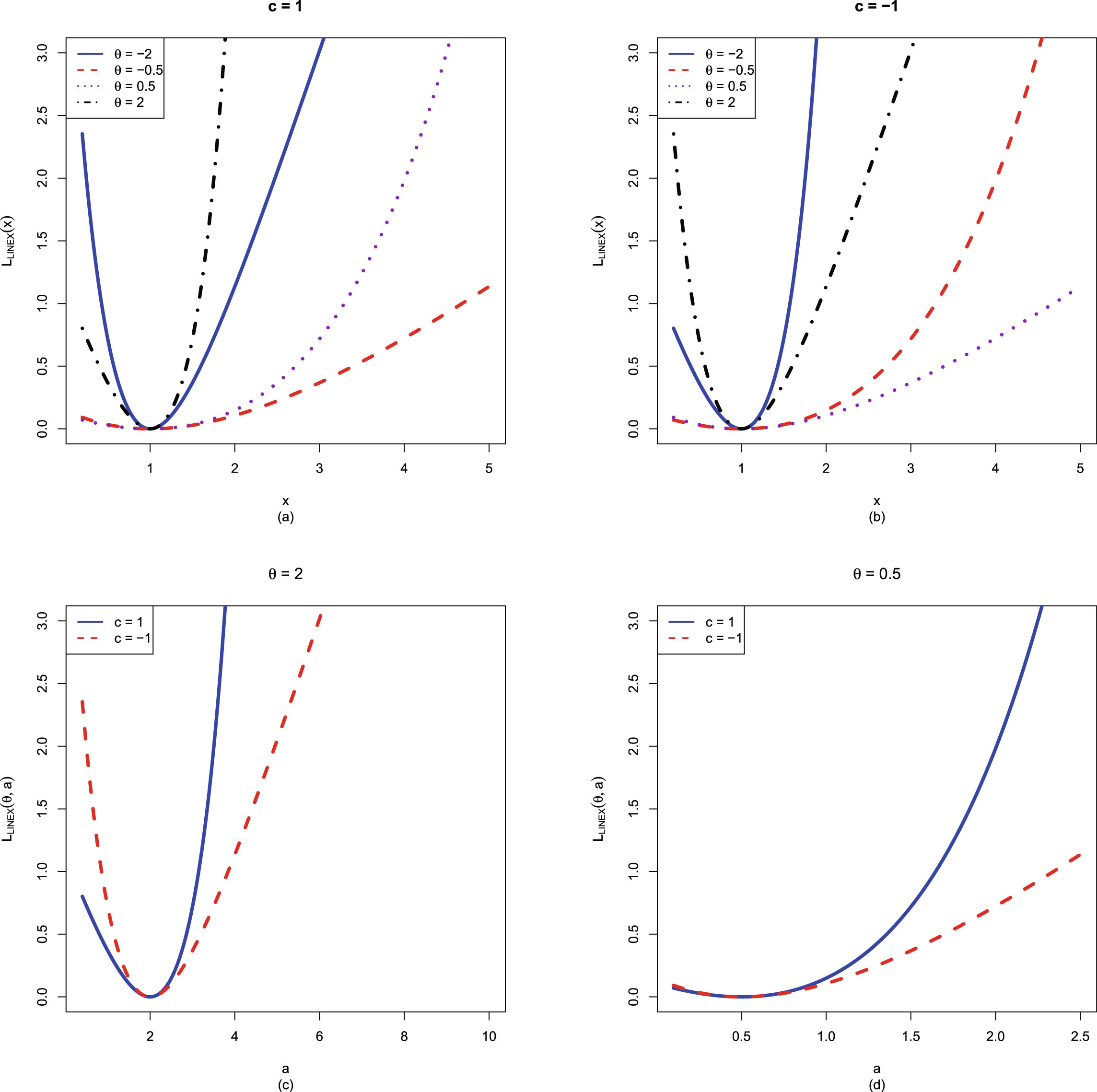
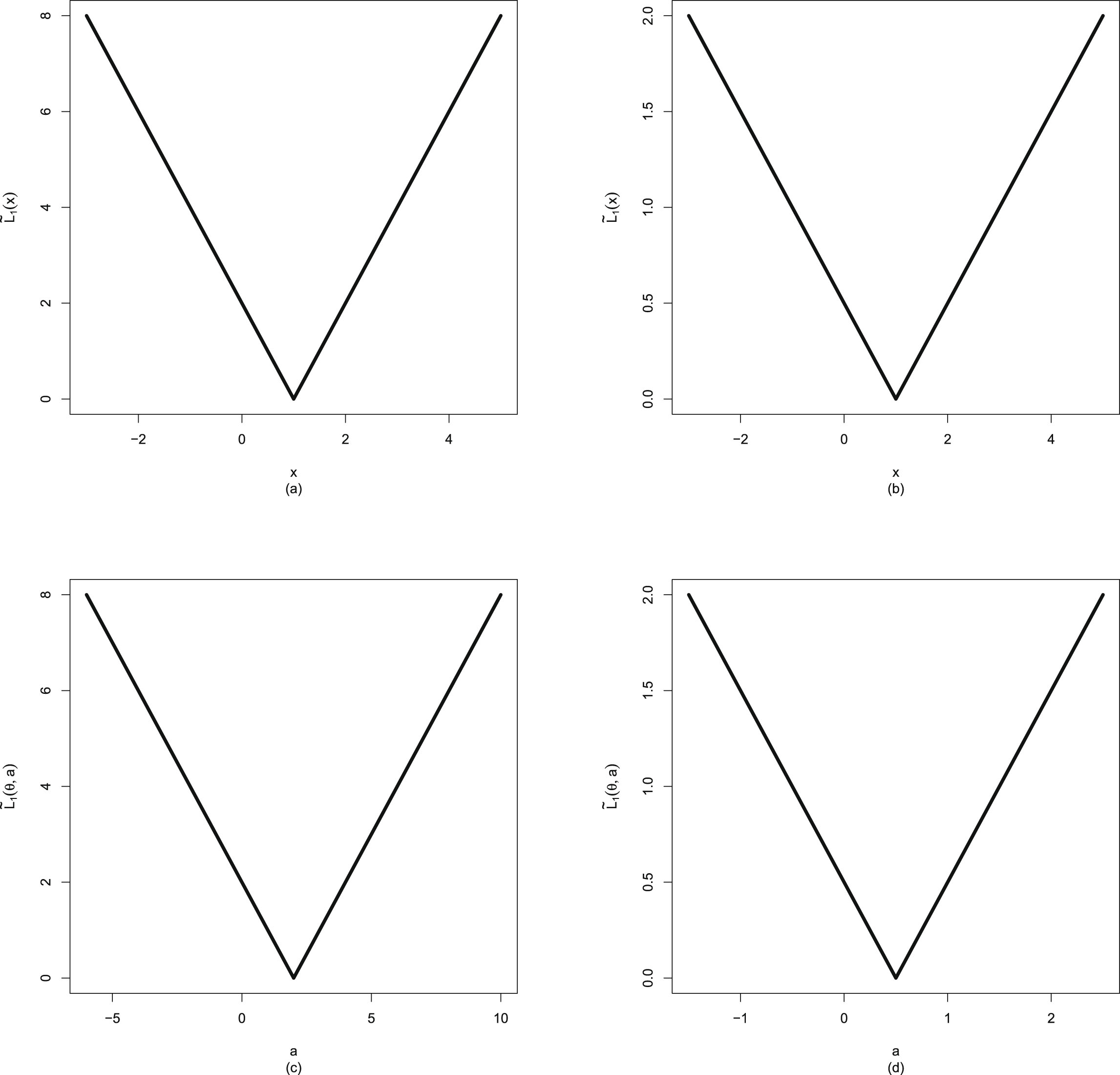
-axis ranges and labels, which are and with a relation . Plots (b) and (d) are the same, with the only difference being the -axis ranges and labels, which are and with a relation .
FIG. 9.7 — SCLF: The LINEX loss function in terms of  and the LINEX loss function in terms of
  and
and  . (a)
. (a)  with
with  and
and  . (b)
. (b)  with
with  and
and  . (c)
. (c)  with
with  and
and  . (d)
. (d)  with
with  and
and  .
.
and the LINEX loss function in terms of and . (a) with and . (b) with and . (c) with and . (d) with and .
FIG. 9.8 — SCLF: The absolute error loss function in terms of  and the absolute error loss function in terms of
  and
and  . (a)
. (a)  with
with  . (b)
. (b)  with
with  . (c)
. (c)  with
with  . (d)
. (d)  with
with  .
.
and the absolute error loss function in terms of and . (a) with . (b) with . (c) with . (d) with .
3. The ranges of  for plots (a) and (b) are
  . The range of
  for plot (c) is
  , as
, as  . The range of
  for plot (d) is
  , as
, as  .
.
for plots (a) and (b) are . The range of for plot (c) is , as . The range of for plot (d) is , as .
9.5.3 Weighted Absolute Error Loss Function
The weighted absolute error loss function in terms of  is given by
 (9.20)
where
(9.20)
where  . Note that
  . The weighted absolute error loss function in terms of
  and
and  is given by
 (9.21)
where
(9.21)
where  and
and  . Note that the weighted absolute error loss function
  has weight
  .
.
is given by
(9.20)
. Note that . The weighted absolute error loss function in terms of and is given by
(9.21)
and . Note that the weighted absolute error loss function has weight .
The weighted absolute error loss function in terms of  and the weighted absolute error loss function in terms of
  and
and  are plotted in figure 9.9. From the figure, we observe the following facts.
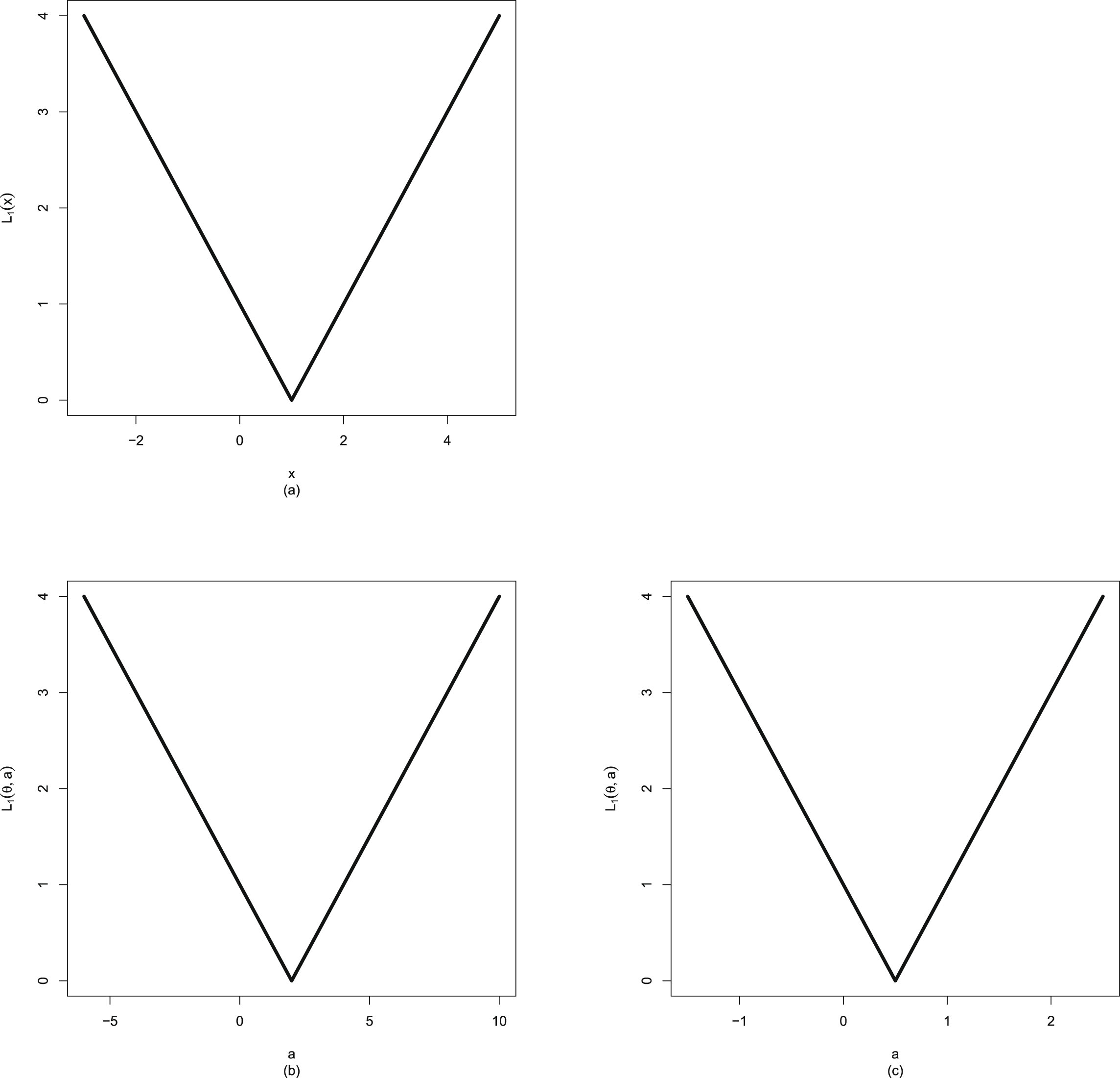
and the weighted absolute error loss function in terms of and are plotted in figure 9.9. From the figure, we observe the following facts.
FIG. 9.9 — SCLF: The weighted absolute error loss function in terms of  and the weighted absolute error loss function in terms of
  and
and  . (a)
. (a)  . (b)
. (b)  with
with  . (c)
. (c)  with
with  .
.
and the weighted absolute error loss function in terms of and . (a) . (b) with . (c) with .
1.  satisfies (a)–(e).
satisfies (a)–(e).
2. Plots (a) and (b) ((a) and (c)) are the same, with the only differences being the  -axis ranges and labels, which are
  and
and  with a relation
  .
.
-axis ranges and labels, which are and with a relation .
3. The range of  for plot (a) is
  . The range of
  for plot (b) is
  , as
, as  . The range of
  for plot (c) is
  , as
, as  .
.
for plot (a) is . The range of for plot (b) is , as . The range of for plot (c) is , as .
9.5.4 Power Loss Function
The power loss function in terms of  is given by
 (9.22)
where
(9.22)
where  ,
,  , and
, and  . It is useful to point out that
  is used to guarantee that
  satisfies (c). Note that
  . The power loss function in terms of
  and
and  is given by
 (9.23)
where
(9.23)
where  .
.
is given by
(9.22)
, , and . It is useful to point out that is used to guarantee that satisfies (c). Note that . The power loss function in terms of and is given by
(9.23)
.
The power loss function,  with
with  , includes the absolute error loss function (
 ) and the squared error loss function (
 ) as special cases.
with , includes the absolute error loss function () and the squared error loss function () as special cases.
9.5.5 Weighted Power Loss Function
The weighted power loss function in terms of  is given by
 (9.24)
where
(9.24)
where  and
and  . Note that
  . The weighted power loss function in terms of
  and
and  is given by
 (9.25)
where
(9.25)
where  and
and  . Note that the weighted power loss function
  has weight
  .
.
is given by
(9.24)
and . Note that . The weighted power loss function in terms of and is given by
(9.25)
and . Note that the weighted power loss function has weight .
The weighted power loss function,  with
with  , includes the weighted absolute error loss function (
 ) and the weighted squared error loss function (
 ) as special cases.
with , includes the weighted absolute error loss function () and the weighted squared error loss function () as special cases.
9.5.6 Log-1 Loss Function
The log-1 loss function in terms of  is given by
 (9.26)
where
(9.26)
where  . Note that
  . The log-1 loss function in terms of
  and
and  is given by
 (9.27)
where
(9.27)
where  .
.
is given by
(9.26)
. Note that . The log-1 loss function in terms of and is given by
(9.27)
.
The log-1 loss function in terms of  and the log-1 loss function in terms of
  and
and  are plotted in figure 9.10. From the figure, we observe the following facts.
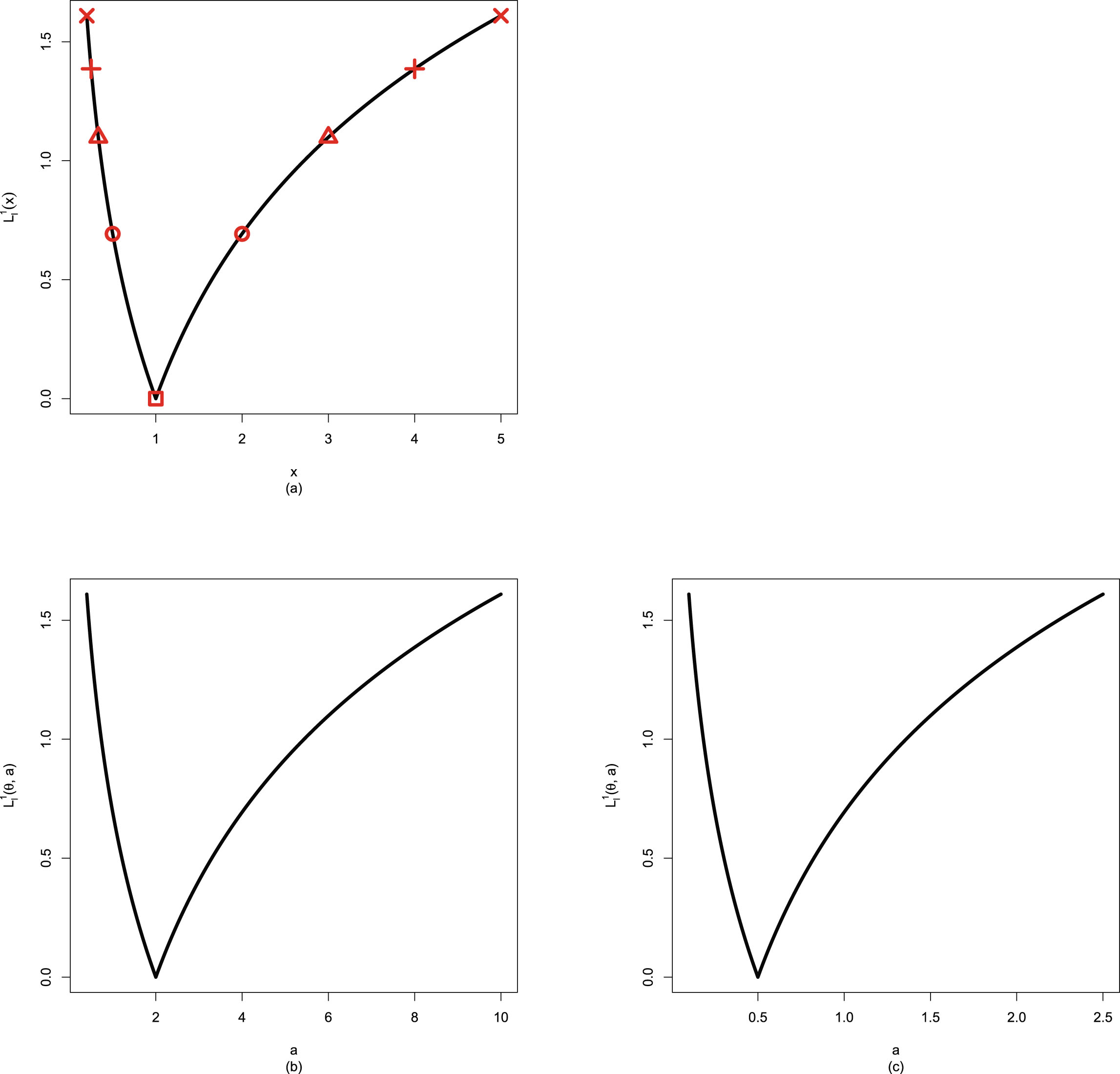
and the log-1 loss function in terms of and are plotted in figure 9.10. From the figure, we observe the following facts.
FIG. 9.10 — SCLF: The log-1 loss function in terms of  and the log-1 loss function in terms of
  and
and  . (a)
. (a)  . (b)
. (b)  with
with  . (c)
. (c)  with
with  .
.
and the log-1 loss function in terms of and . (a) . (b) with . (c) with .
1.  satisfies (a)–(d), and (g) with
  .
.
satisfies (a)–(d), and (g) with .
2. We place the same markers on
 for
for  in plot (a). We see from plot (a) that the loss function
  has balanced convergence rates or penalties for
  large and small, which means that property (g) holds.
in plot (a). We see from plot (a) that the loss function has balanced convergence rates or penalties for large and small, which means that property (g) holds.
3. Plots (a) and (b) ((a) and (c)) are the same, with the only differences being the  -axis ranges and labels, which are
  and
and  with a relation
  .
.
-axis ranges and labels, which are and with a relation .
4. The range of  for plot (a) is
  . The range of
  for plot (b) is
  , as
, as  . The range of
  for plot (c) is
  , as
, as  .
.
for plot (a) is . The range of for plot (b) is , as . The range of for plot (c) is , as .
9.5.7 Log-2 Loss Function
The log-2 loss function in terms of  is given by
 (9.28)
where
(9.28)
where  . Note that
  . The log-2 loss function in terms of
  and
and  is given by
 (9.29)
where
(9.29)
where  .
.
is given by
(9.28)
. Note that . The log-2 loss function in terms of and is given by
(9.29)
.
The log-2 loss function in terms of  and the log-2 loss function in terms of
  and
and  are plotted in figure 9.11. From the figure, we observe the following facts.
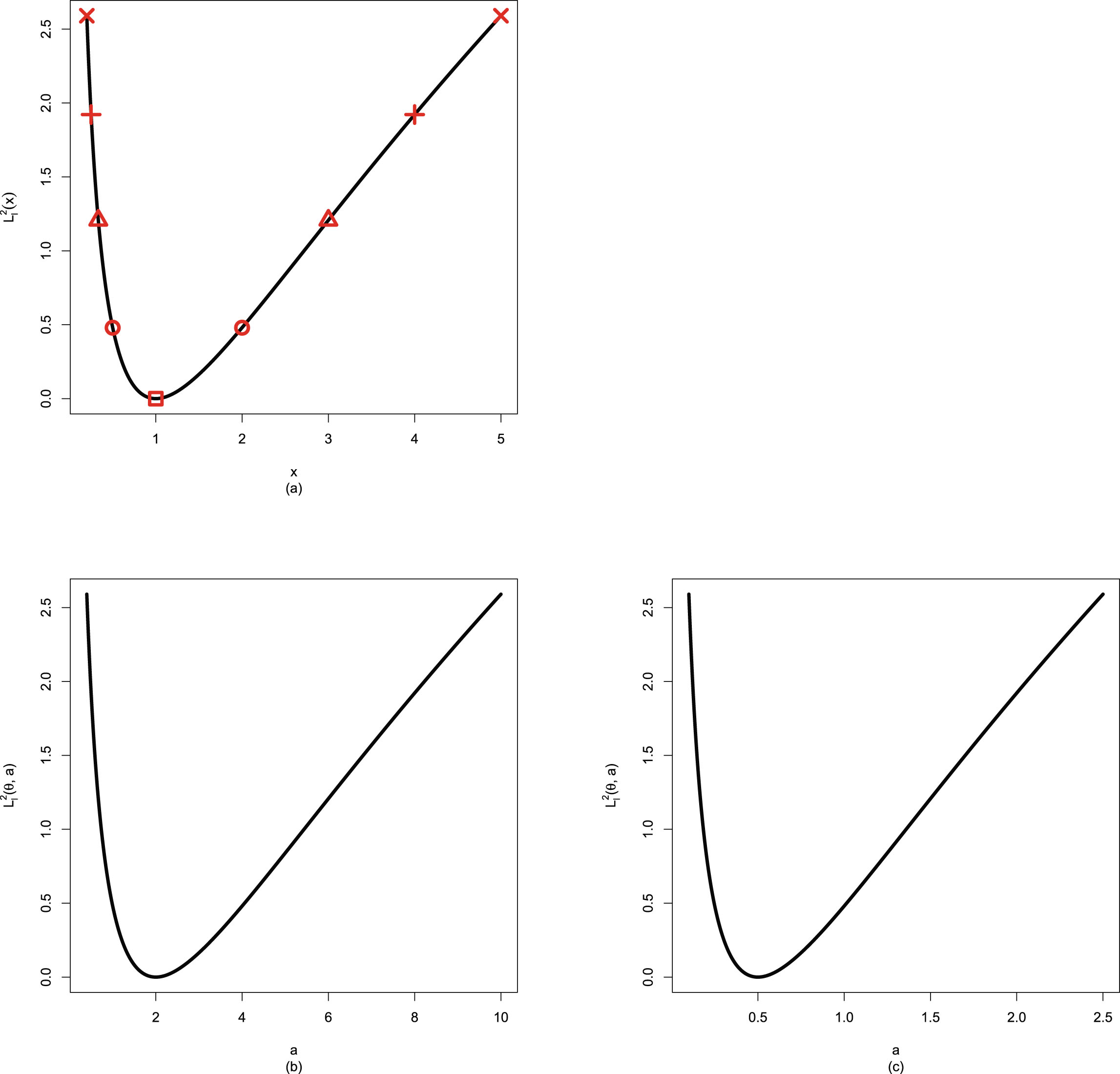
and the log-2 loss function in terms of and are plotted in figure 9.11. From the figure, we observe the following facts.
FIG. 9.11 — SCLF: The log-2 loss function in terms of  and the log-2 loss function in terms of
  and
and  . (a)
. (a)  . (b)
. (b)  with
with  . (c)
. (c)  with
with  .
.
and the log-2 loss function in terms of and . (a) . (b) with . (c) with .
1.  satisfies (a)–(d), (f), and (g) with
  .
.
satisfies (a)–(d), (f), and (g) with .
2. We place the same markers on
 for
for  in plot (a). We see from plot (a) that the loss function
  has balanced convergence rates or penalties for
  large and small, which means that property (g) holds.
in plot (a). We see from plot (a) that the loss function has balanced convergence rates or penalties for large and small, which means that property (g) holds.
3. Plots (a) and (b) ((a) and (c)) are the same, with the only differences being the  -axis ranges and labels, which are
  and
and  with a relation
  .
.
-axis ranges and labels, which are and with a relation .
4. The range of  for plot (a) is
  . The range of
  for plot (b) is
  , as
, as  . The range of
  for plot (c) is
  , as
, as  .
.
for plot (a) is . The range of for plot (b) is , as . The range of for plot (c) is , as .
9.5.8 Generalized Log Loss Function
The generalized log loss function (see Brown (1968)) in terms of  is given by
 (9.30)
where
(9.30)
where  and
and  . Note that
  . The generalized log loss function in terms of
  and
and  is given by
 (9.31)
where
(9.31)
where  and
and  .
.
is given by
(9.30)
and . Note that . The generalized log loss function in terms of and is given by
(9.31)
and .
The generalized log loss function,  with
with  , includes the log-1 loss function (
 ) and the log-2 loss function (
 ) as special cases.
with , includes the log-1 loss function () and the log-2 loss function () as special cases.
9.5.9 Generalized Stein’s Loss Function
The generalized Stein’s loss function (see Zhang et al. (2023)) in terms of  is given by
 (9.32)
where
(9.32)
where  and
and  . Note that
  . The generalized Stein’s loss function in terms of
  and
and  is given by
 (9.33)
where
(9.33)
where  and
and  .
.
is given by
(9.32)
and . Note that . The generalized Stein’s loss function in terms of and is given by
(9.33)
and .
Stein’s loss function  is a special case of the generalized Stein’s loss function
  with
with  .
.
is a special case of the generalized Stein’s loss function with .
The generalized Stein’s loss function in terms of  and the generalized Stein’s loss function in terms of
  and
and  are plotted in figure 9.12. From the figure, we observe the following facts.
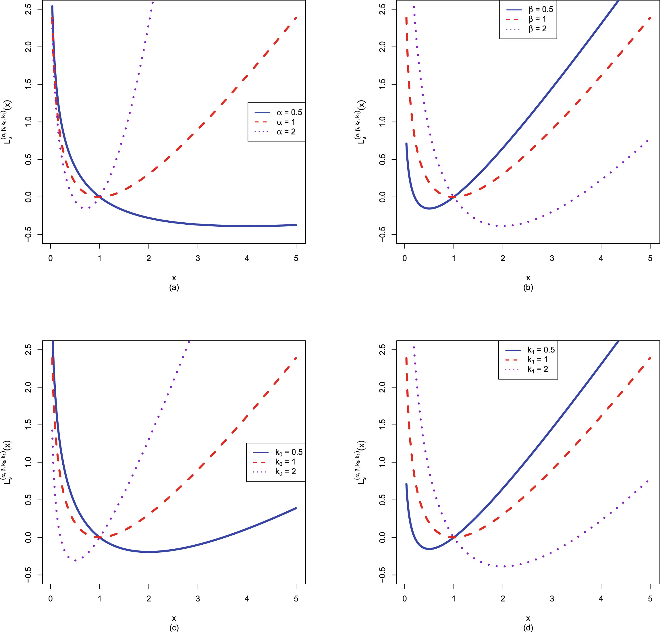

and the generalized Stein’s loss function in terms of and are plotted in figure 9.12. From the figure, we observe the following facts.
FIG. 9.12 — SCLF: The generalized Stein’s loss function in terms of  and the generalized Stein’s loss function in terms of
  and
and  . (a)
. (a)  with
with  and
and  . (b)
. (b)  with
with  and
and  . (c)
. (c)  with
with  and
and  . (d)
. (d)  with
with  and
and  .
.
and the generalized Stein’s loss function in terms of and . (a) with and . (b) with and . (c) with and . (d) with and .
1.  satisfies (a) for
  , (b)–(f) for
  .
.
satisfies (a) for , (b)–(f) for .
2. The ranges of  for the four plots are
  . The ranges of
  for the four plots are
  .
.
for the four plots are . The ranges of for the four plots are .
3. For plot (a) with  ,
,  for all
  when
when  . However, when
  or 2,
or 2,  may be less than 0. This is because

, for all when . However, when or 2, may be less than 0. This is because
But
 and
and

We know that when  , then
  satisfies (f),
  , and this property ensures that
  satisfies (a),
  for all
  .
.
, then satisfies (f), , and this property ensures that satisfies (a), for all .
4. Similarly, for plots (b)–(d),  for all
  when
when  . However, when
  ,
,  , or
, or  ,
,  may be less than 0, because now
for all when . However, when , , or , may be less than 0, because now
From figure 9.12, we see that  for all
  only when
  . In figure 9.13, we will plot the generalized Stein’s loss function in terms of
  and the generalized Stein’s loss function in terms of
  and
and  for three parameter sets
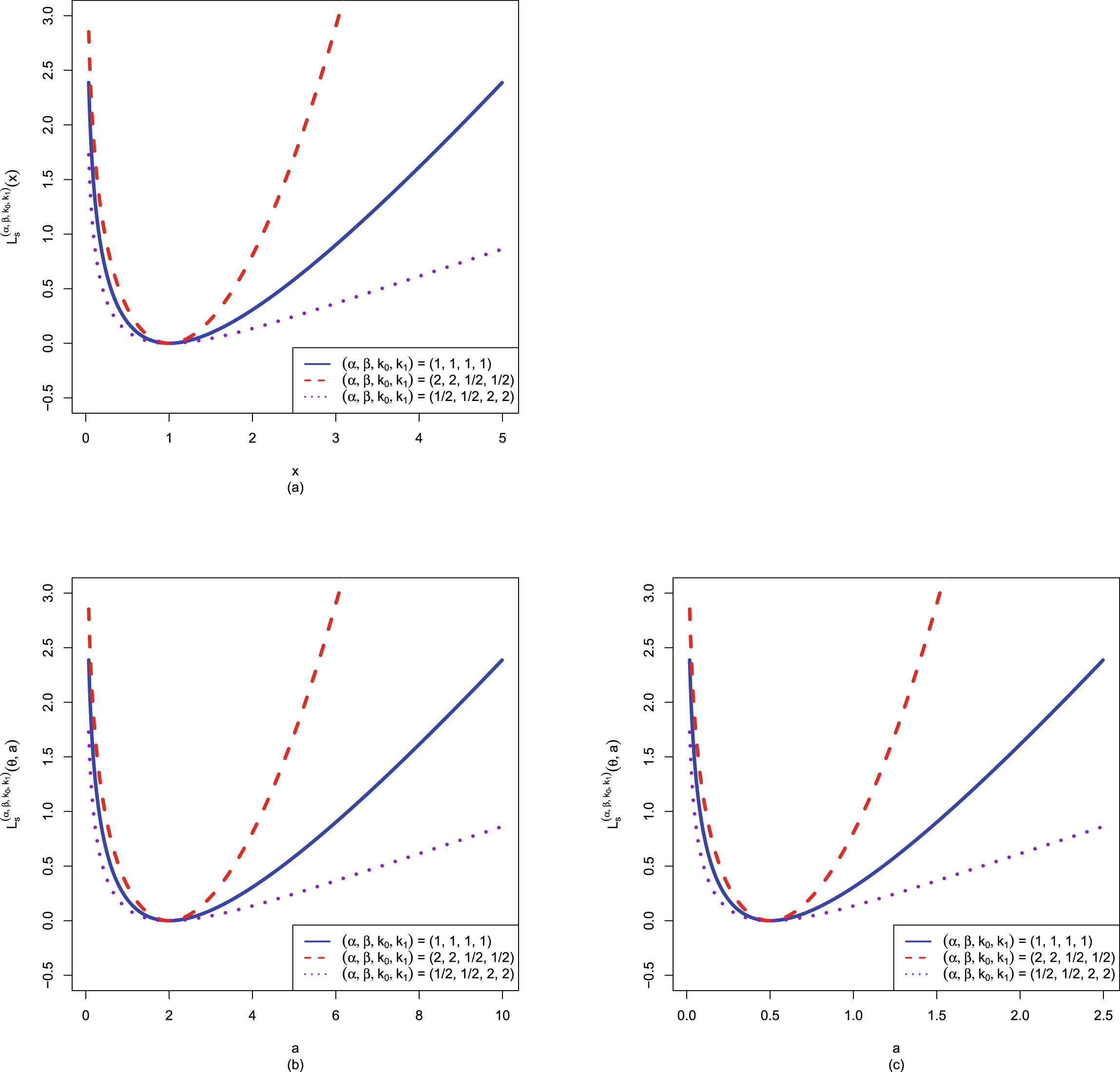
 so that the parameters satisfy
  . From the figure, we observe the following facts.
for all only when . In figure 9.13, we will plot the generalized Stein’s loss function in terms of and the generalized Stein’s loss function in terms of and for three parameter sets
FIG. 9.13 — SCLF: The generalized Stein’s loss function in terms of  and the generalized Stein’s loss function in terms of
  and
and  . (a)
. (a)  with
with  . (b)
. (b)  with
with  and
and  . (c)
. (c)  with
with  and
and  .
.
and the generalized Stein’s loss function in terms of and . (a) with . (b) with and . (c) with and .
. From the figure, we observe the following facts.
1.  satisfies (a) for
  , (b)–(f) for
  .
.
satisfies (a) for , (b)–(f) for .
2. Plots (a) and (b) ((a) and (c)) are the same, with the only differences being the  -axis ranges and labels, which are
  and
and  with a relation
  .
.
-axis ranges and labels, which are and with a relation .
3. The range of  for plot (a) is
  . The range of
  for plot (b) is
  , as
, as  . The range of
  for plot (c) is
  , as
, as  .
.
for plot (a) is . The range of for plot (b) is , as . The range of for plot (c) is , as .
4. Stein’s loss function  is a special case of the generalized Stein’s loss function
  with
with  . However, the generalized Stein’s loss function
  is more flexible than Stein’s loss function
  by changing the parameter values of
  , while keeping
  .
.
is a special case of the generalized Stein’s loss function with . However, the generalized Stein’s loss function is more flexible than Stein’s loss function by changing the parameter values of , while keeping .
9.5.10 Generalized Power-Power Loss Function
The generalized power-power loss function (see Zhang et al. (2023)) in terms of  is given by
 (9.34)
where
(9.34)
where  and
and  . Note that
  . The generalized power-power loss function in terms of
  and
and  is given by
 (9.35)
where
(9.35)
where  and
and  .
.
is given by
(9.34)
and . Note that . The generalized power-power loss function in terms of and is given by
(9.35)
and .
The power-power loss function  is a special case of the generalized power-power loss function
  with
with  .
.
is a special case of the generalized power-power loss function with .
The generalized power-power loss function in terms of  and the generalized power-power loss function in terms of
  and
and  are plotted in figure 9.14. From the figure, we observe the following facts.
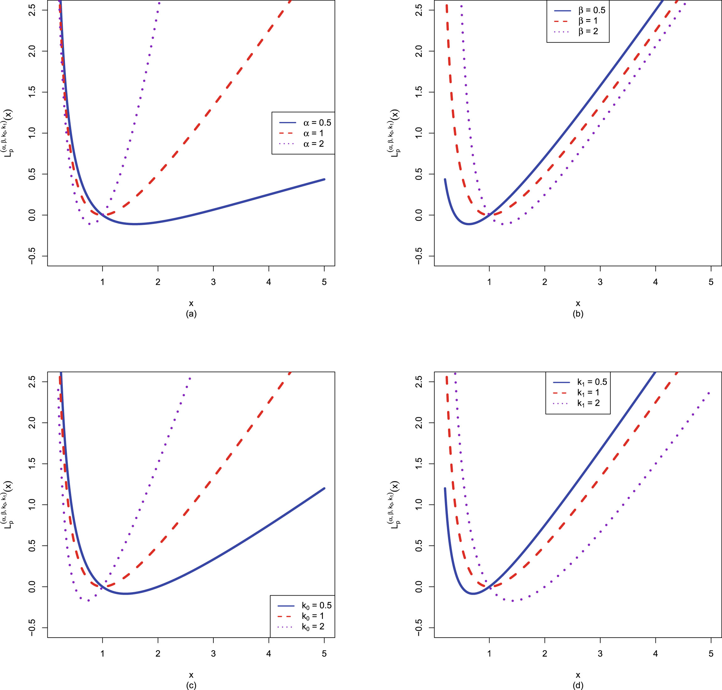

and the generalized power-power loss function in terms of and are plotted in figure 9.14. From the figure, we observe the following facts.
FIG. 9.14 — SCLF: The generalized power-power loss function in terms of  and the generalized power-power loss function in terms of
  and
and  . (a)
. (a)  with
with  and
and  . (b)
. (b)  with
with  and
and  . (c)
. (c)  with
with  and
and  . (d)
. (d)  with
with  and
and  .
.
and the generalized power-power loss function in terms of and . (a) with and . (b) with and . (c) with and . (d) with and .
1.  satisfies (a) for
  , (b)–(f) for
  , and (g) with
  .
.
satisfies (a) for , (b)–(f) for , and (g) with .
2. The ranges of  for the four plots are
  . The ranges of
  for the four plots are
  .
.
for the four plots are . The ranges of for the four plots are .
3. For plot (a) with  ,
,  for all
  when
when  . However, when
  or 2,
or 2,  may be less than 0. This is because

, for all when . However, when or 2, may be less than 0. This is because
But
 and
and

We know that when  , then
  satisfies (f),
  , and this property ensures that
  satisfies (a),
  for all
  .
.
, then satisfies (f), , and this property ensures that satisfies (a), for all .
4. Similarly, for plots (b)–(d),  for all
  when
when  . However, when
  ,
,  , or
, or  ,
,  may be less than 0, because now
for all when . However, when , , or , may be less than 0, because now
From figure 9.14, we see that  for all
  only when
  . In figure 9.15, we will plot the generalized power-power loss function in terms of
  and the generalized power-power loss function in terms of
  and
and  for three parameter sets
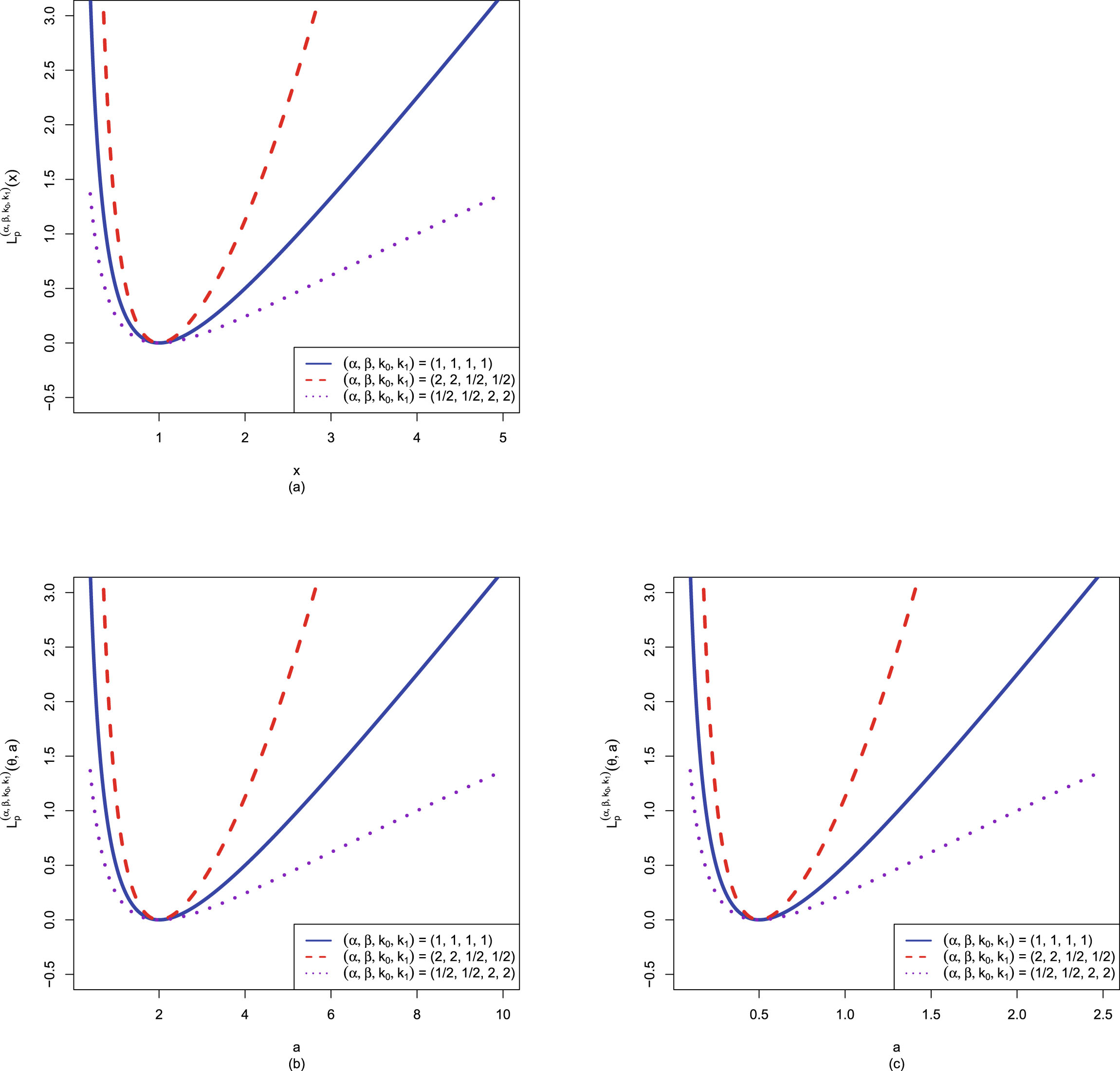
 so that the parameters satisfy
  . From the figure, we observe the following facts.
for all only when . In figure 9.15, we will plot the generalized power-power loss function in terms of and the generalized power-power loss function in terms of and for three parameter sets
FIG. 9.15 — SCLF: The generalized power-power loss function in terms of  and the generalized power-power loss function in terms of
  and
and  . (a)
. (a)  with
with  . (b)
. (b)  with
with  and
and  . (c)
. (c)  with
with  and
and  .
.
and the generalized power-power loss function in terms of and . (a) with . (b) with and . (c) with and .
. From the figure, we observe the following facts.
1.  satisfies (a) for
  , (b)–(f) for
  , and (g) with
  .
.
satisfies (a) for , (b)–(f) for , and (g) with .
2. Plots (a) and (b) ((a) and (c)) are the same, with the only differences being the  -axis ranges and labels, which are
  and
and  with a relation
  .
.
-axis ranges and labels, which are and with a relation .
3. The range of  for plot (a) is
  . The range of
  for plot (b) is
  , as
, as  . The range of
  for plot (c) is
  , as
, as  .
.
for plot (a) is . The range of for plot (b) is , as . The range of for plot (c) is , as .
4. The power-power loss function  is a special case of the generalized power-power loss function
  with
with  . However, the generalized power-power loss function
  is more flexible than the power-power loss function
  by changing the parameter values of
  , while keeping
  .
.
is a special case of the generalized power-power loss function with . However, the generalized power-power loss function is more flexible than the power-power loss function by changing the parameter values of , while keeping .
9.6 Summary of the Loss Functions
In this section, we will give a summary of the loss functions.
The forms and comments of some loss functions which are meaningful on  are given in table 9.4. From the table, we have the following observations.


are given in table 9.4. From the table, we have the following observations.
TAB. 9.4 — SCLF: The forms and comments of some loss functions which are meaningful on  .
.
.
| Loss functions |  |
 |
Comments on  |
| LINEX |  |
 |
(e), (f) |
 |
 |
 |
(e) |
 |
 |
 |
(e), (f) |
 |
 |
 |
(e),  |
| Absolute error |  |
 |
(e) |
| Squared error |  |
 |
(e), (f) |
| Power |  |
 |
(e),  |
| log-1 |  |
 |
(d), (g) with  |
| log-2 |  |
 |
 |
 |
 |
 |
 |
| Stein’s |  |
 |
 |
| (Generalized Stein’s) |  |
 |
 |
| Power–power |  |
 |
 |
| (Generalized power–power) |  |
 |
 |
1. All the loss functions have properties (a)–(c).
2. The weighted power loss function,  with
with  , includes the weighted absolute error loss function (
 ) and the weighted squared error loss function (
 ) as special cases.
with , includes the weighted absolute error loss function () and the weighted squared error loss function () as special cases.
3. The power loss function,  with
with  , includes the absolute error loss function (
 ) and the squared error loss function (
 ) as special cases.
with , includes the absolute error loss function () and the squared error loss function () as special cases.
4. The power loss function in Zhang et al. (2023) is the weighted power loss function in this book; The absolute error loss function in Zhang et al. (2023) is the weighted absolute error loss function in this book; The squared error loss function in Zhang et al. (2023) is the weighted squared error loss function in this book. We are sorry for the inconvenience.
5. The generalized log loss function,  with
with  , includes the log-1 loss function (
 ) and the log-2 loss function (
 ) as special cases.
with , includes the log-1 loss function () and the log-2 loss function () as special cases.
6. Stein’s loss function  is a special case of the generalized Stein’s loss function
  with
with  .
.
is a special case of the generalized Stein’s loss function with .
7. The power-power loss function  is a special case of the generalized power-power loss function
  with
with  .
.
is a special case of the generalized power-power loss function with .
8. The weighted power loss functions (and thus  and
and  ) do not have properties (d) and (g), since
and ) do not have properties (d) and (g), since
9. The power loss functions (and thus  and
and  ) do not have properties (d) and (g), since
and ) do not have properties (d) and (g), since
10. The weighted power loss functions  , the power loss functions
  , and the generalized log loss functions for odd
  do not have property (f). Moreover, they are not differentiable at
  .
.
, the power loss functions , and the generalized log loss functions for odd do not have property (f). Moreover, they are not differentiable at .
11. The generalized log loss functions do not have property (e), since they are convex to the left of  (
( for
for  ,
,  for
for  ,
,  ) and concave to the right of
  .
.
( for , for , ) and concave to the right of .
12. The following loss functions have both properties (c) and (d), and thus they penalize gross overestimation and gross underestimation equally, that is, an action  will incur an infinite loss when it tends to 0 or
  : log-1, log-2, generalized log, Stein’s, generalized Stein’s, power-power, and generalized power-power.
will incur an infinite loss when it tends to 0 or : log-1, log-2, generalized log, Stein’s, generalized Stein’s, power-power, and generalized power-power.
13. Stein’s loss function and the generalized Stein’s loss function have properties (d)–(f). However, they have unbalanced convergence rates or penalties for  too large and
  too small.
too large and too small.
14. The power-power loss function and the generalized power-power loss function have properties (d)–(g). They have balanced convergence rates or penalties for  too large and
  too small. That is, they have all seven properties of a good loss function on
  .
.
too large and too small. That is, they have all seven properties of a good loss function on .
15. The power-log loss function and Zhang’s loss function are defined on  , and thus they are not listed in this table.
, and thus they are not listed in this table.
Chapter 10 Summaries and Discussions
In this chapter, we will give some summaries and discussions of the book.
1. For a hierarchical model (1.1), we calculate the posterior density  and the marginal density
  . Since
  is a positive parameter in the model (1.1), the Bayes estimator of
  under the squared error loss function is not appropriate. In contrast, we should choose Stein’s loss function because it penalizes gross overestimation and gross underestimation equally, that is, an action
  will incur an infinite loss when it tends to 0 or
  . After that, we calculate the Bayes estimators of
  (
( and
and  and the PESLs of
 and
and  ).
).
and the marginal density . Since is a positive parameter in the model (1.1), the Bayes estimator of under the squared error loss function is not appropriate. In contrast, we should choose Stein’s loss function because it penalizes gross overestimation and gross underestimation equally, that is, an action will incur an infinite loss when it tends to 0 or . After that, we calculate the Bayes estimators of ( and and the PESLs of and ).
2. In order to calculate the empirical Bayes estimators of the positive parameter  , we must calculate the estimators of the hyperparameters of the model (1.1). The estimators of the hyperparameters of the model (1.1) by the moment method and their consistencies are summarized in a theorem. Moreover, the estimators of the hyperparameters of the model (1.1) by the MLE method and their consistencies are summarized in another theorem. Finally, the empirical Bayes estimators of the positive parameter
  of the model (1.1) under Stein’s loss function by the moment method and the MLE method are summarized in yet another theorem.
, we must calculate the estimators of the hyperparameters of the model (1.1). The estimators of the hyperparameters of the model (1.1) by the moment method and their consistencies are summarized in a theorem. Moreover, the estimators of the hyperparameters of the model (1.1) by the MLE method and their consistencies are summarized in another theorem. Finally, the empirical Bayes estimators of the positive parameter of the model (1.1) under Stein’s loss function by the moment method and the MLE method are summarized in yet another theorem.
3. We carry out the numerical simulations for the hierarchical model (1.1) in the simulations section in at least four aspects. First, we have exemplified the two inequalities of the Bayes estimators and the PESLs. Second, we have illustrated that the moment estimators and the MLEs are consistent estimators of the hyperparameters. Third, we have calculated the goodness-of-fit of the hierarchical model (1.1) to the simulated data. Fourth, we have plotted the marginal pdfs/pmfs of the hierarchical model (1.1) for various hyperparameters.
4. Numerical results indicate that the MLE method is better than the moment method when estimating the hyperparameters in terms of consistency, goodness-of-fit, Bayes estimators, and PESLs (or posterior Stein’s risks). However, nothing comes for free. Compared to the moment estimators, the MLEs have a heavier computational burden, suffer from numerical instability, require positivity of some hyperparameters in all the iteration processes, and have no analytical solutions. Note also that the MLEs of the hyperparameters are very sensitive to the initial estimators, and the moment estimators are usually proven to be good initial estimators. Moreover, if there is any case where MLE does not exist, then we have a good reason to take moment estimators.
5. In empirical Bayes analysis, the hyperparameters are unknown, and the marginal distribution is used to estimate the hyperparameters from the observations. There are two common methods to estimate the hyperparameters by exploiting the marginal distribution: the moment method and the MLE method. In this book, we use the two methods to estimate the hyperparameters of the hierarchical model (1.1).
6. Comparing the two Bayes estimators  and
and  , we prefer the former one, not because it is larger or smaller than the latter one, but because Stein’s loss function is more appropriate than the squared error loss function for the positive parameter
  , as Stein’s loss function penalizes gross overestimation and gross underestimation equally for
  , while the squared error loss function does not.
and , we prefer the former one, not because it is larger or smaller than the latter one, but because Stein’s loss function is more appropriate than the squared error loss function for the positive parameter , as Stein’s loss function penalizes gross overestimation and gross underestimation equally for , while the squared error loss function does not.
7. Now we present some future works. One may consider extending the hierarchical model (1.1) to different types of non-conjugate priors for the positive parameter of the model (see Berger et al. (2015); Berger (1985, 2006) and the references therein). In these situations, one may not obtain analytical solutions; then one should be able to derive the estimators numerically.
8. For the positive parameter of the hierarchical model (1.1), one may consider using the power-power loss function  which has the property that
  and
and  tend to
  at the same rate, that is,
  has balanced convergence rates or penalties for
  too large and
  too small. The power-power loss function satisfies all seven properties for a good loss function on
  . Therefore, the power-power loss function is recommended to use for the positive parameter space
  .
.
which has the property that and tend to at the same rate, that is, has balanced convergence rates or penalties for too large and too small. The power-power loss function satisfies all seven properties for a good loss function on . Therefore, the power-power loss function is recommended to use for the positive parameter space .
9. Note that in theorems of MLEs, we only stated that the estimators of the hyperparameters of the hierarchical model (1.1) by the MLE method are the solutions to some equations. We can exploit Newton’s method to solve the equations and to numerically obtain the MLEs of the hyperparameters. However, we can not prove the existence and uniqueness of the solutions to our system. The interested readers who have such knowledge and skills are encouraged to solve this issue.
10. In general, the analytical calculations of the MLEs of the hyperparameters by solving some equations are impossible, and thus, we have to resort to numerical solutions. In this book, we exploit Newton’s method to solve the equations and to numerically obtain the MLEs of the hyperparameters. One may consider utilizing the Expectation–Maximization (EM) algorithm to numerically obtain the MLEs of the hyperparameters.
Appendix A: Some Technical Derivations
In this appendix, we will give some technical derivations of the results in chapters 2–8.
A.1 IG-IG: The Proof of Theorem 2.1
In this section, we will prove Theorem 2.1.
First, we derive the posterior density of  . By the Bayes Theorem, we have

. By the Bayes Theorem, we have
It is easy to see that
 for
for  and
and  , and
, and

and , and
Therefore,
 where
where

Second, we derive the marginal density of  . By straightforward calculations, the marginal density of
  is
is

. By straightforward calculations, the marginal density of is
Now recognizing the integrand of the above integral as a kernel of the inverse gamma distribution
 we have

The proof of the theorem is complete. 
A.2 IG-IG: The Proof of Theorem 2.2
In this section, we will prove Theorem 2.2.
Now, let us derive the moment estimators of the hyperparameters ( ,
,  , and
, and  ) of model (2.1). The first three moments of
  are respectively given by

 and
and
 which can be obtained by iterated expectation. More specifically,
 where
where
 and
and

, , and ) of model (2.1). The first three moments of are respectively given by
Note that the pdf of the  distribution integrates to 1, that is,
 (A.1)
(A.1)
distribution integrates to 1, that is,
(A.1)
Moreover,
 where
where
 and
and

Furthermore,
 where
where
 and
and

The moment estimators of  ,
,  , and
, and  are calculated by equating the population moments to the sample moments, that is,
 (A.2)
(A.2)
 (A.3)
(A.3)
 (A.4)
where
(A.4)
where  ,
,  , is the sample
  th moment of
  . Substituting (A.2) into (A.3) and (A.3) into (A.4), we obtain
 (A.5)
(A.5)
 (A.6)
(A.6)
 (A.7)
(A.7)
, , and are calculated by equating the population moments to the sample moments, that is,
(A.2)
(A.3)
(A.4)
, , is the sample th moment of . Substituting (A.2) into (A.3) and (A.3) into (A.4), we obtain
(A.5)
(A.6)
(A.7)
Substituting (A.5) into (A.6) and (A.7), we obtain

We can first solve the above equations for  , and then for
  . After some tedious calculations, we obtain
 (A.8)
(A.8)
 (A.9)
(A.9)
, and then for . After some tedious calculations, we obtain
(A.8)
(A.9)
Substituting (A.8) and (A.9) into (A.5), we obtain
 (A.10)
(A.10)
Finally, the moment estimators of  ,
,  , and
, and  are given by (A.8)–(A.10).
, , and are given by (A.8)–(A.10).
Now, let us show that the moment estimators are consistent estimators of the hyperparameters. It is easy to show that
 for
for  , where
  means convergence in probability. Hence,

, where means convergence in probability. Hence,
Therefore,


The proof of the theorem is complete. 
A.3 IG-IG: The Proof of Theorem 2.3
In this section, we will prove Theorem 2.3.
Proof. The marginal density of  is given by (2.3). Then the likelihood function of
  ,
,  , and
, and  is
is

is given by (2.3). Then the likelihood function of , , and is
Consequently, the log-likelihood function of  ,
,  , and
, and  is
is

, , and is
Taking partial derivatives with respect to  ,
,  , and
, and  and setting them to zeros, we obtain

, , and and setting them to zeros, we obtain
Since
 which can be directly calculated in R software by digamma(x) (R Core Team (2023)), after some algebra, the above equations reduce to

The Jacobian matrix of  ,
,  , and
, and  is given by
 where
where


, , and is given by
Note that
 which can be directly calculated in R software by trigamma(x) (R Core Team (2023)).
We can exploit Newton’s method to solve the equations (2.13)–(2.15) and to numerically obtain the MLEs of  ,
,  , and
, and  . The iterative scheme of Newton’s method is
 where
where  is the Jacobian matrix of
  , and
, and  . Note that the MLEs of
  ,
,  , and
, and  are very sensitive to the initial estimators, and the moment estimators are usually proved to be good initial estimators.
, , and . The iterative scheme of Newton’s method is
is the Jacobian matrix of , and . Note that the MLEs of , , and are very sensitive to the initial estimators, and the moment estimators are usually proved to be good initial estimators.
Now, let us show that the MLEs are consistent estimators of the hyperparameters. From Theorem 10.1.6 in Casella and Berger (2002), we know that the MLEs are consistent estimators of the hyperparameters under some regularity conditions in Miscellanea 10.6.2 in Casella and Berger (2002). The regularity conditions are listed below:
(C1). We observe  , where
  are iid.
, where are iid.
(C2). The parameter is identifiable; that is, if  , then
  .
.
, then .
(C3). The densities  have common support, and
  is differentiable in
  ,
,  , and
, and  .
.
have common support, and is differentiable in , , and .
(C4). The parameter space  contains an open set
  of which the true parameter value
  is an interior point.
contains an open set of which the true parameter value is an interior point.
It remains to show that the marginal density  satisfies all the regularity conditions.
satisfies all the regularity conditions.
First, (C1) is satisfied, as  is a random sample from
  .
.
is a random sample from .
Second, let us show that (C2) is satisfied. The parameter is identifiable
 (A.11)
(A.11)
We have
 (A.12)
(A.12)
Note that
 and thus

Therefore, (A.12) is equivalent to

 which is equivalent to the following equations
 (A.13)
 (A.14)
 (A.15)
(A.13)
(A.14)
(A.15)
From (A.14), we obtain
 (A.16)
(A.16)
Substituting (A.16) into (A.15), we have


Hence,

Consequently, (A.11) is correct, and (C2) is satisfied.
Third, (C3) is satisfied, as the densities  have common support
  , and
, and  is differentiable in
  ,
,  , and
, and  .
.
have common support , and is differentiable in , , and .
Finally, (C4) is satisfied, as the true parameter value
 which is an open set.
Therefore, the marginal density  satisfies all the regularity conditions, and the MLEs are consistent estimators of the hyperparameters.
satisfies all the regularity conditions, and the MLEs are consistent estimators of the hyperparameters.
The proof of the theorem is complete. 
A.4 IG-IG: The Simulation Design of subsection 2.3.2
The simulation design of subsection 2.3.2 is detailed as follows.
We will use these notations.
 is the
  th entry of the matrix
  .
.
 is the
  th row of the matrix
  .
.
 is the
  th column of the matrix
  .
.
 is a zero matrix of size
  .
.
is the th entry of the matrix .
is the th row of the matrix .
is the th column of the matrix .
is a zero matrix of size .
The simulation design consists of the following five steps.
Step 1. Initialization.
 ,
,  ,
,  ,
,  (1e4, 2e4, 4e4, 8e4),
Step 2. Simulate the samples.
 # Allocate a zero matrix for
  .
.
For  from 1 to
  do
do
from 1 to do
set.seed( ) # Set the random seed.
) # Set the random seed.
generate  from
from  #
#  is a vector of length 8e4.
from # is a vector of length 8e4.
generate  from
from  #
#  is a vector of length 8e4.EndFor
from # is a vector of length 8e4.EndFor
Step 3. Compute the moment estimators and the MLEs of the hyperparameters  ,
,  , and
, and  .
.
, , and .
alpha_1 = beta_1 = v_1 = alpha_2 = beta_2 = v_2 = 
For  from 1 to 4 do.
from 1 to 4 do.
 # The
# The  th component of
  .
.
alpha_1_beta_1_v_1 = alpha_2_beta_2_v_2 = 
For  from 1 to
  do
do
from 1 to do
 #
#  is the sample. It is the
  th row,
  th columns of the matrix
  .
.
alpha_1_beta_1_v_1  holds the moment estimators of
  ,
,  , and
, and  computed from
  .
.
holds the moment estimators of , , and computed from .
alpha_2_beta_2_v_2  holds the MLEs of
  ,
,  , and
, and  computed from
  by Newton’s method with the initial estimators being the moment estimators alpha_1_beta_1_v_1
  .
.
holds the MLEs of , , and computed from by Newton’s method with the initial estimators being the moment estimators alpha_1_beta_1_v_1 .
EndFor.
alpha_1  = alpha_1_beta_1_v_1
= alpha_1_beta_1_v_1
beta_1  = alpha_1_beta_1_v_1
= alpha_1_beta_1_v_1
v_1  = alpha_1_beta_1_v_1
= alpha_1_beta_1_v_1
alpha_2  = alpha_2_beta_2_v_2
= alpha_2_beta_2_v_2
beta_2  = alpha_2_beta_2_v_2
= alpha_2_beta_2_v_2
v_2  = alpha_2_beta_2_v_2
= alpha_2_beta_2_v_2
EndFor.
Step 4. Calculate the absolute errors.
Abs_alpha_1 =  # A matrix of size
  .
.
# A matrix of size .
Abs_beta_1 = 
Abs_v_1 = 
Abs_alpha_2 = 
Abs_beta_2 = 
Abs_v_2 = 
Step 5. Calculate the frequencies of the moment estimators and the MLEs.
F = 
F1 = F2 = 
# the moment estimators

F1

= apply(X = (Abs_alpha_1  =
=  ), MARGIN = 1, FUN = mean) # Compute the frequencies of the moment estimators of
  efficiently using the R built-in function apply().
= ), MARGIN = 1, FUN = mean) # Compute the frequencies of the moment estimators of efficiently using the R built-in function apply().
F1

= apply(X = (Abs_beta_1  =
=  ), MARGIN = 1, FUN = mean)
= ), MARGIN = 1, FUN = mean)
F1 

= apply(X = (Abs_v_1  =
=  ), MARGIN = 1, FUN = mean)
= ), MARGIN = 1, FUN = mean)
F = F1
= F1

= F1
F1

= apply(X = (Abs_alpha_1  =
=  ), MARGIN = 1, FUN = mean)
= ), MARGIN = 1, FUN = mean)
F1

= apply(X = (Abs_beta_1  =
=  ), MARGIN = 1, FUN = mean)
= ), MARGIN = 1, FUN = mean)
F1

= apply(X = (Abs_v_1  =
=  ), MARGIN = 1, FUN = mean)
= ), MARGIN = 1, FUN = mean)
F = F1
= F1

= F1
F1

= apply(X = (Abs_alpha_1  =
=  ), MARGIN = 1, FUN = mean)
= ), MARGIN = 1, FUN = mean)
F1

= apply(X = (Abs_beta_1  =
=  ), MARGIN = 1, FUN = mean)
= ), MARGIN = 1, FUN = mean)
F1

= apply(X = (Abs_v_1  =
=  ), MARGIN = 1, FUN = mean)
= ), MARGIN = 1, FUN = mean)
F = F1
= F1
= F1
# the MLEs

F2

= apply(X = (Abs_alpha_2  =
=  ), MARGIN = 1, FUN = mean) # Compute the frequencies of the MLEs of
  efficiently using the R built-in function apply().
= ), MARGIN = 1, FUN = mean) # Compute the frequencies of the MLEs of efficiently using the R built-in function apply().
F2

= apply(X = (Abs_beta_2  =
=  ), MARGIN = 1, FUN = mean)
= ), MARGIN = 1, FUN = mean)
F2

= apply(X = (Abs_v_2  =
=  ), MARGIN = 1, FUN = mean)
= ), MARGIN = 1, FUN = mean)
F = F2
= F2

= F2
F2

= apply(X = (Abs_alpha_2  =
=  ), MARGIN = 1, FUN = mean)
= ), MARGIN = 1, FUN = mean)
F2

= apply(X = (Abs_beta_2  =
=  ), MARGIN = 1, FUN = mean)
= ), MARGIN = 1, FUN = mean)
F2

= apply(X = (Abs_v_2  =
=  ), MARGIN = 1, FUN = mean)
= ), MARGIN = 1, FUN = mean)
F = F2
= F2

= F2
F2

= apply(X = (Abs_alpha_2  =
=  ), MARGIN = 1, FUN = mean)
= ), MARGIN = 1, FUN = mean)
F2

= apply(X = (Abs_beta_2  =
=  ), MARGIN = 1, FUN = mean)
= ), MARGIN = 1, FUN = mean)
F2

= apply(X = (Abs_v_2  =
=  ), MARGIN = 1, FUN = mean)
= ), MARGIN = 1, FUN = mean)
F = F2
= F2
= F2
The simulation design is complete. 
A.5 G-G: The Proof of Theorem 3.1
In this section, we will prove Theorem 3.1.
First, we derive the posterior density of  . By the Bayes Theorem, we have

. By the Bayes Theorem, we have
It is easy to see that
 for
for  and
and  , and
, and

and , and
Therefore,
 where
where

Second, we derive the marginal density of  . By straightforward calculations, the marginal density of
  is
is

. By straightforward calculations, the marginal density of is
Now recognizing the integrand of the above integral as a kernel of the gamma distribution, we have

The proof of the theorem is complete. 
A.6 G-G: The Calculations of
In this section, we will calculate  and the two PESLs
  and
and  .
.
and the two PESLs and .
First, let us calculate  . For the sake of simplicity, the *’s are dropped from
  and
and  . We have
 where
where
 is the digamma function.
. For the sake of simplicity, the *’s are dropped from and . We have
Second, let us calculate  and
and  . We have
 and
and

and . We have
The calculations are complete. 
A.7 G-G: The Proof of Theorem 3.2
In this section, we will prove Theorem 3.2.
Now, let us derive the moment estimators of the hyperparameters ( ,
,  , and
, and  ) of model (3.1). The first three moments of
  are respectively given by

 and
and
 which can be obtained by iterated expectation. More specifically, for
  ,
,
 where
where
 and
and

, , and ) of model (3.1). The first three moments of are respectively given by
,
Note that the pdf of the  distribution integrates to 1, that is,

 (A.17)
distribution integrates to 1, that is,
(A.17)
Moreover, for  ,
,
 where
where
 and
and

,
Furthermore, for  ,
,
 where
where
 and
and

,
The moment estimators of  ,
,  , and
, and  are calculated by equating the population moments to the sample moments, that is,
 (A.18)
 (A.19)
 (A.20)
where
(A.20)
where  ,
,  , is the sample
  th moment of
  . Substituting (A.18) into (A.19) and (A.19) into (A.20), we obtain
 (A.21)
 (A.22)
 (A.23)
, , and are calculated by equating the population moments to the sample moments, that is,
(A.18)
(A.19)
(A.20)
, , is the sample th moment of . Substituting (A.18) into (A.19) and (A.19) into (A.20), we obtain
(A.21)
(A.22)
(A.23)
Substituting (A.21) into (A.22) and (A.23), we obtain


We can first solve the above equations for  , and then for
  . After some tedious calculations, we obtain
 (A.24)
 (A.25)
, and then for . After some tedious calculations, we obtain
(A.24)
(A.25)
Substituting (A.24) and (A.25) into (A.21), we obtain
 (A.26)
(A.26)
Finally, the moment estimators of  ,
,  , and
, and  are given by (A.24)–(A.26).
, , and are given by (A.24)–(A.26).
Now, let us show that the moment estimators are consistent estimators of the hyperparameters. It is easy to show that
 for
for  , where
  means convergence in probability. Hence,

, where means convergence in probability. Hence,
Therefore,


The proof of the theorem is complete. 
A.8 G-G: The Proof of Theorem 3.3
In this section, we will prove Theorem 3.3.
The marginal density of  is
is
 for
for  and
and  , where
  is the gamma function. Then the likelihood function of
  ,
,  , and
, and  is
is

is
and , where is the gamma function. Then the likelihood function of , , and is
Consequently, the log-likelihood function of  ,
,  , and
, and  is
is

, , and is
Taking partial derivatives with respect to  ,
,  , and
, and  and setting them to zeros, we obtain

, , and and setting them to zeros, we obtain
Since
 which can be directly calculated in R software by digamma(x) (R Core Team (2023)), after some algebra, the above equations reduce to

The Jacobian matrix of  ,
,  , and
, and  is given by
 where
where


, , and is given by
Therefore,  is a real symmetric matrix. Note that
 which can be directly calculated in R software by trigamma(x) (R Core Team (2023)).
is a real symmetric matrix. Note that
We can exploit Newton’s method to solve the equations (3.13)–(3.15) and to numerically obtain the MLEs of  ,
,  , and
, and  . The iterative scheme of Newton’s method is
 where
where  is the Jacobian matrix of
  , and
, and  . Note that the MLEs of
  ,
,  , and
, and  are very sensitive to the initial estimators, and the moment estimators are usually proven to be good initial estimators.
, , and . The iterative scheme of Newton’s method is
is the Jacobian matrix of , and . Note that the MLEs of , , and are very sensitive to the initial estimators, and the moment estimators are usually proven to be good initial estimators.
Now, let us show that the MLEs are consistent estimators of the hyperparameters. From Theorem 10.1.6 in Casella and Berger (2002), we know that the MLEs are consistent estimators of the hyperparameters under some regularity conditions in Miscellanea 10.6.2 in Casella and Berger (2002). The regularity conditions are listed below:
(C1). We observe  , where
  are iid.
, where are iid.
(C2). The parameter is identifiable; that is, if  , then
  .
.
, then .
(C3). The densities  have common support, and
  is differentiable in
  ,
,  , and
, and  .
.
have common support, and is differentiable in , , and .
(C4). The parameter space  contains an open set
  of which the true parameter value
  is an interior point.
contains an open set of which the true parameter value is an interior point.
It remains to show that the marginal density  satisfies all the regularity conditions. Let
  be the support set of
  .
.
satisfies all the regularity conditions. Let be the support set of .
First, (C1) is satisfied, as  is a random sample from
  .
.
is a random sample from .
Second, let us show that (C2) is satisfied. The parameter is identifiable

 (A.27)
(A.27)
We have
 (A.28)
(A.28)
Note that
 and thus

Therefore, (A.28) is equivalent to

 which is equivalent to the following equations
 (A.29)
 (A.30)
 (A.31)
(A.29)
(A.30)
(A.31)
From (A.30), we obtain
 (A.32)
(A.32)
Substituting (A.32) into (A.31), we have


Hence,

Consequently, (A.27) is correct, and (C2) is satisfied.
Third, (C3) is satisfied, as the densities  have common support
  , and
, and  is differentiable in
  ,
,  , and
, and  .
.
have common support , and is differentiable in , , and .
Finally, (C4) is satisfied, as the true parameter value
 which is an open set.
Therefore, the marginal density  satisfies all the regularity conditions, and the MLEs are consistent estimators of the hyperparameters.
satisfies all the regularity conditions, and the MLEs are consistent estimators of the hyperparameters.
The proof of the theorem is complete. 
A.9 Exp-IG: The Proof of Theorem 4.1
In this section, we will prove Theorem 4.1.
First, let us derive the posterior density of  . By the Bayes Theorem, we have

. By the Bayes Theorem, we have
It is easy to see that
 for
for  and
and  , and
, and

and , and
Therefore,
 where
where

Second, let us derive the marginal density of  . By straightforward calculations, the marginal density of
  is
is

. By straightforward calculations, the marginal density of is
The proof of the theorem is complete. 
A.10 Exp-IG: The Proof of Theorem 4.2
In this section, we will prove Theorem 4.2.
The first two moments of  can be obtained by iterated expectation. More specifically,
 for
for  , and
, and
 for
for  .
.
can be obtained by iterated expectation. More specifically,
, and
.
The moment estimators of  and
and  are calculated by equating the population moments to the sample moments, that is,
 (A.33)
 (A.34)
where
(A.34)
where  ,
,  , is the sample
  th moment of
  . Substituting (A.33) into (A.34), we obtain

and are calculated by equating the population moments to the sample moments, that is,
(A.33)
(A.34)
, , is the sample th moment of . Substituting (A.33) into (A.34), we obtain
We can first solve the above equations for  , and then for
  , and obtain
 which are the moment estimators of
  and
and  .
.
, and then for , and obtain
and .
Now, let us show that the moment estimators are consistent estimators of the hyperparameters. It is easy to show that
 for
for  , where
  means convergence in probability. Hence,

, where means convergence in probability. Hence,
Therefore,
 and
and

The proof of the theorem is complete. 
A.11 Exp-IG: The Proof of Theorem 4.3
In this section, we will prove Theorem 4.3.
The marginal density of  is
is
 for
for  and
and  . Then the likelihood function of
  and
and  is
is

is
and . Then the likelihood function of and is
Consequently, the log-likelihood function of  and
and  is
is

and is
Taking partial derivatives with respect to  and
and  and setting them to zeros, we obtain

and and setting them to zeros, we obtain
After some algebraic operations, the above equations reduce to

Moreover, the Jacobian matrix of  and
and  is given by
 where
where

and is given by
We can exploit Newton’s method to solve the equations (4.14) and (4.15) and to obtain the MLEs of  and
and  . The iterative scheme of Newton’s method is
 where
where  is the Jacobian matrix of
  and
and  . Note that the MLEs of
  and
and  are very sensitive to the initial estimators, and the moment estimators are usually proved to be good initial estimators.
and . The iterative scheme of Newton’s method is
is the Jacobian matrix of and . Note that the MLEs of and are very sensitive to the initial estimators, and the moment estimators are usually proved to be good initial estimators.
Now, let us show that the MLEs are consistent estimators of the hyperparameters. From Theorem 10.1.6 in Casella and Berger (2002), we know that the MLEs are consistent estimators of the hyperparameters under some regularity conditions in Miscellanea 10.6.2 in Casella and Berger (2002). The regularity conditions are listed below:
(C1). We observe  , where
  are iid.
, where are iid.
(C2). The parameter is identifiable; that is, if  , then
  .
.
, then .
(C3). The densities  have common support, and
  is differentiable in
  and
and  .
.
have common support, and is differentiable in and .
(C4). The parameter space  contains an open set
  of which the true parameter value
  is an interior point.
contains an open set of which the true parameter value is an interior point.
It remains to show that the marginal density  satisfies all the regularity conditions. Let
  be the support set of
  .
.
satisfies all the regularity conditions. Let be the support set of .
First, (C1) is satisfied, as  is a random sample from
  .
.
is a random sample from .
Second, let us show that (C2) is satisfied. The parameter is identifiable
 (A.35)
(A.35)
We have
 (A.36)
(A.36)
Note that
 and thus

Therefore, (A.36) is equivalent to
 which implies
 (A.37)
where
(A.37)
where  is a constant which does not depend on
  . Hence,
 and (A.37) reduces to

(A.37)
is a constant which does not depend on . Hence,
Therefore,

Consequently, (A.35) is correct, and (C2) is satisfied.
Third, (C3) is satisfied, as the densities  have common support
  , and
, and  is differentiable in
  and
and  .
.
have common support , and is differentiable in and .
Finally, (C4) is satisfied, as the true parameter value
 which is an open set.
Therefore, the marginal densities  satisfy all the regularity conditions, and the MLEs are consistent estimators of the hyperparameters.
satisfy all the regularity conditions, and the MLEs are consistent estimators of the hyperparameters.
The proof of the theorem is complete. 
A.12 N-IG: The Proof of Theorem 5.1
In this section, we will prove Theorem 5.1.
By the Bayes Theorem, we have

It is easy to see that
 for
for  and
and  , and
, and

and , and
Therefore,
 where
where

The proof of the theorem is complete. 
A.13 N-IG: The Proof of Lemma 5.1
In this section, we will prove Lemma 5.1.
The proof of the lemma exploits Stein’s lemma (see Lemma 3.6.5 in Casella and Berger (2002)). The first two moments of  are familiar to all. The calculation of
  can be found in Example 3.6.6 in Casella and Berger (2002) and thus it is omitted. Now we calculate
  . We have

are familiar to all. The calculation of can be found in Example 3.6.6 in Casella and Berger (2002) and thus it is omitted. Now we calculate . We have
The proof of the lemma is complete.
A.14 N-IG: The Proof of Lemma 5.2
In this section, we will prove Lemma 5.2.
The expectation and variance of the inverse gamma distribution can be found in Definition B.35 in Jackman (2009), and thus it is omitted. It is easy to calculate

The proof of the lemma is complete.
A.15 N-IG: The Proof of Lemma 5.3
In this section, we will prove Lemma 5.3.
By straightforward calculations, the marginal density of  is
is

is
Now recognizing the integrand of the above integral as a kernel of the inverse gamma distribution
 we have

The proof of the lemma is complete.
A.16 N-IG: The Proof of Lemma 5.4
In this section, we will prove Lemma 5.4.
We will use the iterated expectation identity and Lemmas 5.1–5.3. Note that  ,
,  , and
, and  are known hyperparameters. By Lemmas 5.1 and 5.3, we have


, , and are known hyperparameters. By Lemmas 5.1 and 5.3, we have
By Lemmas 5.2 and 5.3, we have


Therefore, we have

The proof of the lemma is complete.
A.17 N-IG: The Proof of Theorem 5.2
In this section, we will prove Theorem 5.2.
The hyperparameters of the model are  ,
,  , and
, and  . By Lemma 5.3, we know that the marginal distribution of the model is a non-standardized Student-t distribution, that is,

, , and . By Lemma 5.3, we know that the marginal distribution of the model is a non-standardized Student-t distribution, that is,
Since there are three hyperparameters, if we want to obtain the estimators of the hyperparameters of the model by the moment method, we need to calculate the first three moments of  at least. By Lemma 5.4, we obtain the first four population moments of
  as follows. Furthermore, letting the population moments be equal to the sample moments, we obtain
 where
where
 is the sample
  th moment of
  . Let
. Let

at least. By Lemma 5.4, we obtain the first four population moments of as follows. Furthermore, letting the population moments be equal to the sample moments, we obtain
th moment of . Let
Note that the first three moments of  involve only two unknown parameters
  and
and  , and thus the two parameters are over-determined. Therefore, we use the first, second, and fourth moments of
  to determine the three parameters
  ,
,  , and
, and  . Note that
 (A.38)
involve only two unknown parameters and , and thus the two parameters are over-determined. Therefore, we use the first, second, and fourth moments of to determine the three parameters , , and . Note that
(A.38)
Substituting (A.38) into the expressions of the first, second, and fourth moments of  , we obtain
 (A.39)
, we obtain
(A.39)
Therefore, the moment estimator of  is
is
 (A.40)
is
(A.40)
Substituting (A.40) into (A.39) and simplifying, we have
 (A.41)
 (A.42)
(A.41)
(A.42)
Note that equation (A.42) is equivalent to
 (A.43)
(A.43)
Substituting (A.41) into (A.43) and simplifying, we obtain
 (A.44)
(A.44)
Dividing (A.41) by (A.44) and solving for  , we obtain that the moment estimator of
  is
is
 (A.45)
, we obtain that the moment estimator of is
(A.45)
Substituting (A.45) into (A.41) and simplifying, we obtain that the moment estimator of  is
is
 (A.46)
is
(A.46)
Consequently, the moment estimators of the hyperparameters of the model are given by (A.40), (A.45), and (A.46).
Now, let us show that the moment estimators are consistent estimators of the hyperparameters. It is easy to show that
 for
for  , where
  means convergence in probability. Hence,

, where means convergence in probability. Hence,
Therefore,

 and
and

The proof of the theorem is complete. 
A.18 N-IG: The Proof of Theorem 5.3
In this section, we will prove Theorem 5.3.
Now we derive the MLEs of  ,
,  , and
, and  . The hyperparameters of the model are
  ,
,  , and
, and  . By Lemma 5.3, we know that the marginal distribution of the model is a non-standardized Student-t distribution, that is,
 with a density function
 where
where  is the gamma function. Note that
  ,
,  ,
,  , and
, and  have the relationships given by (A.38). After the change of variables, we obtain

, , and . The hyperparameters of the model are , , and . By Lemma 5.3, we know that the marginal distribution of the model is a non-standardized Student-t distribution, that is,
is the gamma function. Note that , , , and have the relationships given by (A.38). After the change of variables, we obtain
Then the likelihood function of  ,
,  , and
, and  is
is

, , and is
Consequently, the log-likelihood function of  ,
,  , and
, and  is
is

, , and is
Taking partial derivatives with respect to  ,
,  , and
, and  and setting them to zeros, we obtain

, , and and setting them to zeros, we obtain
Since
 which can be directly calculated in R software by digamma(x) (R Core Team (2023)), after some algebra, the above equations reduce to

The Jacobian matrix of  ,
,  , and
, and  is given by
 where
where


, , and is given by
Note that
 which can be directly calculated in R software by trigamma(x) (R Core Team (2023)).
We can exploit Newton’s method to solve the equations (5.11)–(5.13) and to numerically obtain the MLEs of  ,
,  , and
, and  . The iterative scheme of Newton’s method is
 where
where  is the Jacobian matrix of
  , and
, and  . Note that the MLEs of
  ,
,  , and
, and  are very sensitive to the initial estimators, and the moment estimators are usually proved to be good initial estimators.
, , and . The iterative scheme of Newton’s method is
is the Jacobian matrix of , and . Note that the MLEs of , , and are very sensitive to the initial estimators, and the moment estimators are usually proved to be good initial estimators.
Now, let us show that the MLEs are consistent estimators of the hyperparameters. From Theorem 10.1.6 in Casella and Berger (2002), we know that the MLEs are consistent estimators of the hyperparameters under some regularity conditions in Miscellanea 10.6.2 in Casella and Berger (2002). The regularity conditions are listed below:
(C1). We observe  , where
  are iid.
, where are iid.
(C2). The parameter is identifiable; that is, if  , then
  .
.
, then .
(C3). The densities  have common support, and
  is differentiable in
  ,
,  , and
, and  .
.
have common support, and is differentiable in , , and .
(C4). The parameter space  contains an open set
  of which the true parameter value
  is an interior point.
contains an open set of which the true parameter value is an interior point.
It remains to show that the marginal density  satisfies all the regularity conditions.
satisfies all the regularity conditions.
First, (C1) is satisfied, as  is a random sample from
  .
.
is a random sample from .
Second, let us show that (C2) is satisfied. The parameter is identifiable
 (A.47)
(A.47)
We have
 (A.48)
(A.48)
Note that
 and thus

Therefore, (A.48) is equivalent to
 which is equivalent to the following equations

 (A.49)
(A.49)
Note that (A.49)
 (A.50)
 (A.51)
(A.50)
(A.51)
Substituting (A.51) into (A.50), we have

Hence,

Consequently, (A.47) is correct, and (C2) is satisfied.
Third, (C3) is satisfied, as the densities  have common support
  , and
, and  is differentiable in
  ,
,  , and
, and  .
.
have common support , and is differentiable in , , and .
Finally, (C4) is satisfied, as the true parameter value
 which is an open set.
Therefore, the marginal density  satisfies all the regularity conditions, and the MLEs are consistent estimators of the hyperparameters.
satisfies all the regularity conditions, and the MLEs are consistent estimators of the hyperparameters.
The proof of the theorem is complete. 
A.19 N-NIG: The Proof of Theorem 6.1
In this section, we will prove Theorem 6.1.
Let  be the hyperparameters. The marginal distribution of
  in the model (6.2) is

be the hyperparameters. The marginal distribution of in the model (6.2) is
To lighten notations, the  will be dropped in the densities. Some of the following derivations are quoted from Example 1.5.1 (p. 20) of Mao and Tang (2012) and Zhang et al. (2019a).
will be dropped in the densities. Some of the following derivations are quoted from Example 1.5.1 (p. 20) of Mao and Tang (2012) and Zhang et al. (2019a).
For the random variables, parameters, and hyperparameters, their domains are respectively given by
 and
and

By the Bayes Theorem, the joint posterior distribution of  and
and  is
is

and is
The joint conjugate prior distribution of  and
and  is decomposed as
 which is a normal-inverse-gamma distribution. Hence,

and is decomposed as
It is easy to see that

 and
and

Therefore,
 (A.52)
(A.52)
The expression in the square brackets of (A.52) changes to
 where
where

Let
 (A.53)
(A.53)
Then (A.52) reduces to

It is shown that  is a normal-inverse-gamma distribution as follows. The joint posterior distribution
  can be written as
  , where

is a normal-inverse-gamma distribution as follows. The joint posterior distribution can be written as , where
That is,

Therefore, the joint posterior distribution  is
is
 (A.54)
is
(A.54)
The joint prior distribution  is
is
 (A.55)
is
(A.55)
Comparing (A.55) and (A.54), we find that the normal-inverse-gamma distribution is a conjugate prior for  of
of  .
.
of .
Now, let us derive the marginal posterior density of  . We have
 by noting that the integrand of the above integral is the kernel of an inverse gamma distribution
  with
with

. We have
with
Therefore,

Now, let us calculate
 (A.56)
(A.56)
Finally, let us derive the marginal density of  . Combining (A.56) and (A.54), we have

. Combining (A.56) and (A.54), we have
The proof of the theorem is complete. 
A.20 N-NIG: The Proof of Theorem 6.2
In this section, we will prove Theorem 6.2.
The hyperparameters of the model (6.2) are  ,
,  ,
,  , and
, and  . By Theorem 6.1, we know that the marginal distribution of the model (6.2) is a non-standardized Student-t distribution, that is,

, , , and . By Theorem 6.1, we know that the marginal distribution of the model (6.2) is a non-standardized Student-t distribution, that is,
Since there are four hyperparameters, if we want to obtain the estimators of the hyperparameters of the model (6.2) by the moment method, we need to calculate the first four moments of  at least. By Lemma 4 in Zhang et al. (2019a), we obtain the first six population moments of
  as follows. Furthermore, letting the population moments be equal to the sample moments, we obtain

at least. By Lemma 4 in Zhang et al. (2019a), we obtain the first six population moments of as follows. Furthermore, letting the population moments be equal to the sample moments, we obtain
From the first moment of  , we obtain the moment estimator of
  as
as

, we obtain the moment estimator of as
Let

From the second moment of  , we obtain the moment estimator of
  as
as

, we obtain the moment estimator of as
From the third moment of  , we obtain the moment estimator of
  as
as

, we obtain the moment estimator of as
Obviously, the two moment estimators of  are not equal. Therefore, we choose one of them as the moment estimator of
  . For simplicity, we use the moment estimator of
  calculated from
  , and ignore the third equation involving
  . Similarly, the equations involving
  and
and  both have
  and
and  . For simplicity, we use the equation involving
  , and ignore the equation involving
  . To have four equations, we will use the equation involving
  . Therefore, the moment equations become

are not equal. Therefore, we choose one of them as the moment estimator of . For simplicity, we use the moment estimator of calculated from , and ignore the third equation involving . Similarly, the equations involving and both have and . For simplicity, we use the equation involving , and ignore the equation involving . To have four equations, we will use the equation involving . Therefore, the moment equations become
Solving the above moment equations, we obtain
 (A.57)


(A.57)
Let

Since  and
and  appear together in
  , we can not directly obtain the estimators of
  and
and  by the moment method. But we can obtain the estimator of
  by the moment method. In the following, we are interested in obtaining the moment estimators of
  ,
,  , and
, and  . The moment equations involving
  ,
,  , and
, and  become

and appear together in , we can not directly obtain the estimators of and by the moment method. But we can obtain the estimator of by the moment method. In the following, we are interested in obtaining the moment estimators of , , and . The moment equations involving , , and become
Since there are three equations and only two parameters  and
and  , for simplicity, we will only use the first two equations and ignore the third equation. Solving the above first two equations for
  and
and  , we obtain the moment estimators of
  and
and  as
as

and , for simplicity, we will only use the first two equations and ignore the third equation. Solving the above first two equations for and , we obtain the moment estimators of and as
Substituting the expressions of  and
and  , and after some algebra, we obtain the expressions of
  and
and  in terms of
  as
as
 (A.58)
 (A.59)
and , and after some algebra, we obtain the expressions of and in terms of as
(A.58)
(A.59)
Therefore, the moment estimators of  ,
,  , and
, and  are given by (A.57)–(A.59).
, , and are given by (A.57)–(A.59).
Now, let us show that the moment estimators are consistent estimators of the hyperparameters. It is easy to show that
 for
for  , where
  means convergence in probability. Hence,

, where means convergence in probability. Hence,
Therefore,

 and
and

The proof of the theorem is complete. 
A.21 N-NIG: The Proof of Theorem 6.3
In this section, we will prove Theorem 6.3.
Now we derive the MLEs of  ,
,  , and
, and  . By Theorem 6.1, we know that the marginal distribution of
  of the model (6.2) is
 for
for  ,
, ,
,  , and
, and  . Then the likelihood function of
  ,
,  , and
, and  is
is

, , and . By Theorem 6.1, we know that the marginal distribution of of the model (6.2) is
,, , and . Then the likelihood function of , , and is
Consequently, the log-likelihood function of  ,
,  , and
, and  is
is

, , and is
Taking partial derivatives with respect to  ,
,  , and
, and  and setting them to zeros, we obtain

 and
and
 where
where
 which can be directly calculated in R software by digamma(x) (R Core Team (2023)). Let

, , and and setting them to zeros, we obtain
Thus,

After some algebra, the above equations reduce to


In the above equations, the expressions involving  are used for simplifying the R coding.
are used for simplifying the R coding.
We can exploit Newton’s method to solve the above equations and obtain the MLEs of  ,
,  , and
, and  . The iterative scheme of Newton’s method is
 where
where  is the Jacobian matrix of
  and
and  . Note that the MLEs of
  ,
,  , and
, and  are very sensitive to the initial estimators, and the moment estimators are usually proved to be good initial estimators.
, , and . The iterative scheme of Newton’s method is
is the Jacobian matrix of and . Note that the MLEs of , , and are very sensitive to the initial estimators, and the moment estimators are usually proved to be good initial estimators.
The Jacobian matrix of  ,
,  , and
, and  is given by
 where
where


 where
where


, , and is given by
Note that
 which can be directly calculated in R software by trigamma(x) (R Core Team (2023)). In
 , the expressions involving
  are used for simplifying the R coding.
, the expressions involving are used for simplifying the R coding.
Now, let us show that the MLEs are consistent estimators of the hyperparameters. From Theorem 10.1.6 in Casella and Berger (2002), we know that the MLEs are consistent estimators of the hyperparameters under some regularity conditions in Miscellanea 10.6.2 in Casella and Berger (2002). The regularity conditions are listed below:
(C1). We observe  , where
  are iid.
, where are iid.
(C2). The parameter is identifiable; that is, if  , then
  .
.
, then .
(C3). The densities  have common support, and
  is differentiable in
  ,
,  , and
, and  .
.
have common support, and is differentiable in , , and .
(C4). The parameter space  contains an open set
  of which the true parameter value
  is an interior point.
contains an open set of which the true parameter value is an interior point.
It remains to show that the marginal distribution  satisfies all the regularity conditions. Let
  be the support set of
  .
.
satisfies all the regularity conditions. Let be the support set of .
First, (C1) is satisfied, as  is a random sample from
  .
.
is a random sample from .
Second, let us show that (C2) is satisfied. The parameter is identifiable
 (A.60)
(A.60)
We have
 (A.61)
(A.61)
Note that
 and thus

Therefore, (A.61) is equivalent to

 which implies

 (A.62)
where
(A.62)
where  is a constant which does not depend on
  but may depend on
  ,
,  ,
,  ,
,  ,
,  , and
, and  . From (A.62), we obtain
 (A.63)
and
(A.63)
and
 (A.64)
(A.62)
is a constant which does not depend on but may depend on , , , , , and . From (A.62), we obtain
(A.63)
(A.64)
Substituting (A.63) and (A.64) into (A.62), we obtain
 which implies
 (A.65)
(A.65)
Substituting (A.65) into (A.64), we obtain
 (A.66)
(A.66)
Therefore,

Consequently, (A.60) is correct, and (C2) is satisfied.
Third, (C3) is satisfied, as the densities  have common support
  , and
, and  is differentiable in
  ,
,  , and
, and  .
.
have common support , and is differentiable in , , and .
Finally, (C4) is satisfied, as the true parameter value
 which is an open set.
Therefore, the marginal densities  satisfy all the regularity conditions, and the MLEs are consistent estimators of the hyperparameters.
satisfy all the regularity conditions, and the MLEs are consistent estimators of the hyperparameters.
The proof of the theorem is complete. 
A.22 U-IG: The Proof of Theorem 7.1
In this section, we will prove Theorem 7.1.
First, let us prove that the posterior distribution of  is a truncated inverse gamma distribution. By the Bayes Theorem, we have

is a truncated inverse gamma distribution. By the Bayes Theorem, we have
It is easy to see that
 for
for  and
and  . Since
  , we have
 where
where  is the indicator function of
  , which is equal to 1 if
  is true and 0 otherwise. Consequently,
 where
where
 is the kernel of
  .
.
and . Since , we have
is the indicator function of , which is equal to 1 if is true and 0 otherwise. Consequently,
.
In the following, we will derive other forms of  . We have
 (A.67)
. We have
(A.67)
Note that
 is the kernel of the
  distribution, and thus
 (A.68)
where
(A.68)
where  is the pdf of the
  distribution. Substituting (A.68) into (A.67), we obtain

distribution, and thus
(A.68)
is the pdf of the distribution. Substituting (A.68) into (A.67), we obtain
It is easy to calculate the denominator of the above expression as
 which is the cdf of the
  distribution evaluated at
  and it can be numerically computed by utilizing the R built-in function pgamma(). Hence,

distribution evaluated at and it can be numerically computed by utilizing the R built-in function pgamma(). Hence,
That is,  is a truncated inverse gamma distribution on
  . In other words,
  is an inverse gamma distribution
  truncated on
  .
.
is a truncated inverse gamma distribution on . In other words, is an inverse gamma distribution truncated on .
Second, let us derive the marginal pdf of  which is given by
 where the likelihood is
 the prior is
 for
for  and
and  , and
, and
 is the gamma function. Therefore,

which is given by
and , and
It is easy to see that the integrand of the above integral is the kernel of an  distribution, that is,
 for
for  and
and  , or equivalently,

distribution, that is,
and , or equivalently,
Consequently, for  and
and  ,
,
 where
where  is the cdf of the
  distribution.
and ,
is the cdf of the distribution.
The proof of the theorem is complete. 
A.23 U-IG: Some Key Notations and Derivatives
In this section, we will provide some key notations and derivatives.
From Wikipedia (2018a); Geddes et al. (1990); Abramowitz and Stegun (1970), the upper incomplete gamma function is defined as:
 whereas the lower incomplete gamma function is defined as:

They have a simple relationship
 where
where
 is the ordinary gamma function. The normalized lower incomplete gamma function is defined as:
 and the normalized upper incomplete gamma function is defined as:

They have the simple relationship

From Wikipedia (2018a); Geddes et al. (1990), the derivatives of the upper incomplete gamma function  with respect to
  and
and  are given by
 (A.69)
 (A.70)
 (A.71)
where the function
(A.71)
where the function  is a special case of the Meijer G-function (The MathWorks (2018); Geddes et al. (1990)) and it is given by

with respect to and are given by
(A.69)
(A.70)
(A.71)
is a special case of the Meijer G-function (The MathWorks (2018); Geddes et al. (1990)) and it is given by
The derivatives of the function  with respect to
  and
and  are given by (Wikipedia (2018a); Geddes et al. (1990))
 (A.72)
 (A.73)
with respect to and are given by (Wikipedia (2018a); Geddes et al. (1990))
(A.72)
(A.73)
Changing the variables  and
and  to
to  and
and  in (A.69)–(A.73), we obtain the following derivatives
 (A.74)
 (A.75)
 (A.76)
 (A.77)
 (A.78)
and to and in (A.69)–(A.73), we obtain the following derivatives
(A.74)
(A.75)
(A.76)
(A.77)
(A.78)
A.24 U-IG: Tedious and Complicated Calculations of E1,E2,E3
In this section, we will calculate  ,
,  , and
, and  for the hierarchical uniform and inverse gamma model (7.1).
, , and for the hierarchical uniform and inverse gamma model (7.1).
First, let us calculate  . We have

. We have
Note that the integrand of the above integral is the kernel of an  distribution, and thus
 where
where  is the pdf of the
  distribution. Therefore,

distribution, and thus
is the pdf of the distribution. Therefore,
It is easy to calculate the integral in the above numerator as follows:
 which is the cdf of the
  distribution evaluated at
  . Hence,

distribution evaluated at . Hence,
Second, let us calculate  . We have

. We have
The numerator of the above expression is

Note that the integrand of the above integral is the kernel of an  distribution. Therefore, the above expression reduces to
 where
where  is the cdf of the
  distribution evaluated at
  . Hence,

distribution. Therefore, the above expression reduces to
is the cdf of the distribution evaluated at . Hence,
Third, let us calculate  . We have

. We have
The numerator of the above expression is

Let  . Then
  , and
, and

. Then , and
Therefore, the numerator reduces to
 where
where
 and
and

For  , we have
 where
where  is the lower incomplete gamma function and
  is the normalized lower incomplete gamma function. For
  , we have
 where
where  is pdf of the
  distribution, and
 which can be numerically computed by utilizing the R built-in function integrate() very quickly and accurately. Hence,

, we have
is the lower incomplete gamma function and is the normalized lower incomplete gamma function. For , we have
is pdf of the distribution, and
The calculations are complete. 
A.25 U-IG: The Proof of Theorem 7.2
In this section, we will prove Theorem 7.2.
The expectation and variance of  are respectively given by
 and
and

are respectively given by
Next, let us calculate  and
and  . We have
 and
and

and . We have
Therefore,

The moment estimators of  and
and  are calculated by equating the population moments to the sample moments, that is,

 where
where  is the sample first-order moment of
  and
and  is the sample second-order central moment of
  . Solving the above equations, we obtain the moment estimators of
  and
and  :
:


and are calculated by equating the population moments to the sample moments, that is,
is the sample first-order moment of and is the sample second-order central moment of . Solving the above equations, we obtain the moment estimators of and :
Now let us show that the moment estimators are consistent estimators of the hyperparameters. It is easy to show that
 and
and
 where
where  means convergence in probability. Therefore,
 and
and

means convergence in probability. Therefore,
The proof of the theorem is complete. 
A.26 U-IG: The Proof of Theorem 7.3
In this section, we will prove Theorem 7.3.
The likelihood function of  and
and  is
is

and is
Consequently, the log-likelihood function of  and
and  is
is

and is
Taking partial derivatives with respect to  and
and  and setting them to zeros, we obtain


and and setting them to zeros, we obtain
After some algebra, the above equations reduce to


We first need to calculate  . From Wikipedia (2018b), we have
 where
where
 is the upper incomplete gamma function. Hence,

. From Wikipedia (2018b), we have
We can exploit Newton’s method to solve the equations (7.8) and (7.9) and to numerically obtain the MLEs of  and
and  ,
,  and
and  . The iterative scheme of Newton’s method is
 where
where  is the Jacobian matrix of
  and
and  . Note that the MLEs of
  and
and  are very sensitive to the initial estimators, and the moment estimators are usually proved to be good initial estimators.
and , and . The iterative scheme of Newton’s method is
is the Jacobian matrix of and . Note that the MLEs of and are very sensitive to the initial estimators, and the moment estimators are usually proved to be good initial estimators.
The Jacobian matrix of  and
and  is given by
 where
where


and is given by
It remains to calculate


Now we calculate these quantities one by one. We first calculate
 where
where
 is the digamma function. Let
 (A.79)
(A.79)
Then
 (A.80)
(A.80)
Next, we calculate
 where
where

Third, we calculate

 where
where
 is the trigamma function,
  is given by (A.80), and
  is calculated as follows. We have
 where
where

is given by (A.80), and is calculated as follows. We have
Therefore,

Fourth, we calculate
 where
where

Fifth, we calculate
 where
where
 where
where

Hence,

Note that
 (A.81)
(A.81)
From Wikipedia (2018a), we find that

Changing the variables  and
and  to
to  and
and  in the above equation, we arrive at (A.80). Therefore,

and to and in the above equation, we arrive at (A.80). Therefore,
Finally, we calculate
 where
where

Consequently,

Hence,  .
.
.
Now, let us show that the MLEs are consistent estimators of the hyperparameters. From Theorem 10.1.6 in Casella and Berger (2002), we know that the MLEs are consistent estimators of the hyperparameters under some regularity conditions in Miscellanea 10.6.2 in Casella and Berger (2002). The regularity conditions are listed below:
(C1). We observe  , where
  are iid.
, where are iid.
(C2). The parameter is identifiable; that is, if  , then
  for some
  .
.
, then for some .
(C3). The densities  have common support, and
  is differentiable in
  and
and  .
.
have common support, and is differentiable in and .
(C4). The parameter space  contains an open set
  of which the true parameter value
  is an interior point.
contains an open set of which the true parameter value is an interior point.
It remains to show that the marginal density  satisfies all the regularity conditions.
satisfies all the regularity conditions.
First, (C1) is satisfied, as  is a random sample from
  .
.
is a random sample from .
Second, let us show that (C2) is satisfied. The parameter is identifiable

 (A.82)
(A.82)
Note that
 and thus

We have

Taking derivatives with respect to  on both sides of the above equation, we obtain

 which is equivalent to the following equations
 (A.83)
 (A.84)
 (A.85)
on both sides of the above equation, we obtain
(A.83)
(A.84)
(A.85)
From (A.84), we obtain

By (A.85), we have

Hence,

Consequently, (A.82) is correct, and (C2) is satisfied.
Third, (C3) is satisfied, as the densities  have common support
  , and
, and  is differentiable in
  and
and  .
.
have common support , and is differentiable in and .
Finally, (C4) is satisfied, as the true parameter value
 which is an open set.
Therefore, the marginal density  satisfies all the regularity conditions, and the MLEs are consistent estimators of the hyperparameters.
satisfies all the regularity conditions, and the MLEs are consistent estimators of the hyperparameters.
The proof of the theorem is complete. 
A.27 U-IG: The Analytical Calculations of Int
In this section, we will analytically calculate  .
.
.
We have

It remains to calculate  . By (A.69) and (A.70), we have
 since
since

. By (A.69) and (A.70), we have
Therefore,

Consequently,

The calculations are complete. 
A.28 P-G: The Proof of Theorem 8.1
In this section, we will prove Theorem 8.1.
By the Bayes Theorem, the posterior distribution of  is
is

is
It is easy to see that
 and
and

Therefore,
 where
where

Now, let us calculate the marginal pmf of  . We have, for
  and
and  ,
,


. We have, for and ,
In particular, when  is a positive integer, the marginal pmf of
  is
is
 which is a negative binomial distribution, where

is a positive integer, the marginal pmf of is
The proof of the theorem is complete. 
A.29 P-G: The Proof of Theorem 8.2
In this section, we will prove Theorem 8.2.
The hyperparameters of the model (8.1) are  and
and  . To obtain the moment estimators of the hyperparameters of the model (8.1), we need to calculate the first two moments of
  ,
,  and
and  . It is easy to show that

and . To obtain the moment estimators of the hyperparameters of the model (8.1), we need to calculate the first two moments of , and . It is easy to show that
Therefore,
 and
and

Furthermore, letting the population moments be equal to the sample moments, we obtain
 (A.86)
 (A.87)
where
(A.87)
where
 is the sample
  th moment of
  . Substituting (A.86) into (A.87), we obtain

 (A.88)
(A.86)
(A.87)
th moment of . Substituting (A.86) into (A.87), we obtain
(A.88)
Substituting (A.86) into (A.88) and simplifying, we have
 (A.89)
(A.89)
From (A.86) and (A.89), we can solve
 (A.90)
(A.90)
Consequently, the moment estimators of the hyperparameters of the model (8.1) are given by (A.89) and (A.90).
Now, let us show that the moment estimators are consistent estimators of the hyperparameters. It is easy to show that
 for
for  , where
  means convergence in probability. Hence,


, where means convergence in probability. Hence,
Therefore,
 and
and

The proof of the theorem is complete. 
A.30 P-G: The Proof of Theorem 8.3
In this section, we will prove Theorem 8.3.
Now we derive the MLEs of  and
and  . The hyperparameters of the model are
  and
and  . By Theorem 8.1, we know that the marginal distribution of
  of the model (8.1) is
 for
for  and
and  . Then the likelihood function of
  and
and  is
is

and . The hyperparameters of the model are and . By Theorem 8.1, we know that the marginal distribution of of the model (8.1) is
and . Then the likelihood function of and is
Consequently, the log-likelihood function of  and
and  is
is

and is
Taking partial derivatives with respect to  and
and  and setting them to zeros, we obtain

and and setting them to zeros, we obtain
Since
 which can be directly calculated in R software by digamma(x) (R Core Team (2023)), after some algebra, the above equations reduce to

We can exploit Newton’s method to solve the equations (8.12) and (8.13) and to obtain the MLEs of  and
and  . The iterative scheme of Newton’s method is
 where
where  is the Jacobian matrix of
  and
and  . Note that the MLEs of
  and
and  are very sensitive to the initial estimators, and the moment estimators are usually proved to be good initial estimators.
and . The iterative scheme of Newton’s method is
is the Jacobian matrix of and . Note that the MLEs of and are very sensitive to the initial estimators, and the moment estimators are usually proved to be good initial estimators.
The Jacobian matrix of  and
and  is given by
 where
where

and is given by
Note that
 which can be directly calculated in R software by trigamma(x) (R Core Team (2023)).
Now, let us show that the MLEs are consistent estimators of the hyperparameters. From Theorem 10.1.6 in Casella and Berger (2002), we know that the MLEs are consistent estimators of the hyperparameters under some regularity conditions in Miscellanea 10.6.2 in Casella and Berger (2002). The regularity conditions are listed below:
(C1). We observe  , where
  are iid.
, where are iid.
(C2). The parameter is identifiable; that is, if  , then
  .
.
, then .
(C3). The densities  have common support, and
  is differentiable in
  and
and  .
.
have common support, and is differentiable in and .
(C4). The parameter space  contains an open set
  of which the true parameter value
  is an interior point.
contains an open set of which the true parameter value is an interior point.
It remains to show that the marginal distribution  satisfies all the regularity conditions. Let
  be the support set of
  .
.
satisfies all the regularity conditions. Let be the support set of .
First, (C1) is satisfied, as  is a random sample from
  .
.
is a random sample from .
Second, let us show that (C2) is satisfied. The parameter is identifiable
 (A.91)
(A.91)
We have
 (A.92)
(A.92)
Note that
 and thus

Therefore, (A.92) is equivalent to

 which implies

 (A.93)
 (A.94)
where
(A.94)
where  and
and  are constants which do not depend on
  but may depend on
  ,
,  ,
,  , and
, and  . From (A.93), we obtain

(A.93)
(A.94)
and are constants which do not depend on but may depend on , , , and . From (A.93), we obtain
From (A.94), we obtain

Therefore,

Consequently, (A.91) is correct, and (C2) is satisfied.
Third, (C3) is satisfied, as the pmfs  have common support
  , and
, and  is differentiable in
  and
and  .
.
have common support , and is differentiable in and .
Finally, (C4) is satisfied, as the true parameter value
 which is an open set.
Therefore, the marginal pmfs  satisfy all the regularity conditions, and the MLEs are consistent estimators of the hyperparameters.
satisfy all the regularity conditions, and the MLEs are consistent estimators of the hyperparameters.
The proof of the theorem is complete. 
Appendix B: Common Univariate Distributions
In this appendix, we will summarize some basic results on common univariate distributions. This appendix is adapted from “Table of Common Distributions” of Casella and Berger (2002).
B.1 Univariate Continuous Distributions
___________________________________________________________________________________

pdf:
 mean and variance:
 moment generating function (mgf):
 notes:
 is the (complete) beta function.
 is the (complete) gamma function.
___________________________________________________________________________________

pdf:

 mean and variance:
 mgf:
mgf:
 notes:
  is a special case of Student’s
  . Moreover, if
  and
and  are independent standard normal
  , then
  is
is  .
.
is a special case of Student’s . Moreover, if and are independent standard normal , then is .
___________________________________________________________________________________

pdf:
 mean and variance:
 mgf:
mgf:
 notes:
 is a special case of the gamma distribution.

___________________________________________________________________________________

pdf:

 mean and variance:
 mgf:
mgf:
 notes: Also known as the Laplace distribution.
___________________________________________________________________________________

pdf:
 mean and variance:
 mgf:
mgf:
 notes:
 is a special case of the gamma distribution.
  is
is  .
.
is .
___________________________________________________________________________________

pdf:

 mean and variance:

 mgf:
mgf:
 notes:
 where
where  and
and  are independent.
  .
.
and are independent. .
___________________________________________________________________________________

pdf:
 mean and variance:
 mgf:
mgf:
 notes: Some special cases are
 and
and

 is the inverse (inverted) gamma distribution.
___________________________________________________________________________________
 pdf:
pdf:


 , then
  .
.
_______________________________________________________________________________________

pdf:

 mean and variance:
 mgf:
mgf:
 notes: The cdf is given by

 pdf:
pdf:

 mean and variance:
 mgf:
mgf:
 notes:
 is a normal distribution.
_______________________________________________________________________________________

pdf:

 mean and variance:
 mgf:
mgf:
 notes: Sometimes called the Gaussian distribution.
_______________________________________________________________________________________

pdf:
 mean and variance:

 mgf:
mgf:

________________________________________________________________________________________

pdf:

 mean and variance:

 mgf:
mgf:
 notes:
  is the
  distribution.
is the distribution.
________________________________________________________________________________________

pdf:
 mean and variance:
 mgf:
mgf:
 notes: If
  and
and  , this is a special case of the beta distribution,

and , this is a special case of the beta distribution,
_______________________________________________________________________________________

pdf:
 mean and variance:

 mgf: The mgf exists only for
  . Its form is not very useful.
. Its form is not very useful.
notes:
 is the exponential distribution.
 is the Weibull distribution.
_______________________________________________________________________________________
B.2 Univariate Discrete Distributions
_______________________________________________________________________________________

pmf:
 mean and variance:
 mgf:
mgf:
 notes:
 is a special case of the binomial distribution.
_______________________________________________________________________________________

pmf:

 mean and variance:
 mgf:
mgf:
 notes:
 is a Bernoulli distribution.
_______________________________________________________________________________________

pmf:
 mean and variance:
 mgf:
mgf:

______________________________________________________________________________________

pmf:
 mean and variance:
 where
where  .
.
.
mgf:
 notes:
 is a special case of the negative binomial distribution.
_______________________________________________________________________________________

pmf:

 mean and variance:
 notes: If
  and
and  , the range
  will be appropriate.
and , the range will be appropriate.
_______________________________________________________________________________________

pmf:

 mean and variance:
 where
where  .
.
.
mgf:
 notes: The random variable
  counts the number of failures before the
  th success. An alternative form of the pmf is given by


counts the number of failures before the th success. An alternative form of the pmf is given by
The random variable  is the trial at which the
  th success occurs. The random variable
  .
.
 is the geometric distribution.
is the trial at which the th success occurs. The random variable .
_______________________________________________________________________________________

pmf:
 mean and variance:
 mgf:
mgf:

__________________________________________________________________________________________
References
Abramowitz M., Stegun I. A. (1970) Handbook of mathematical functions, 9th edn. United States Government Printing Office, New York.
Adler D., Murdoch D., others (2017) rgl: 3D visualization using OpenGL. R package version 0.98.1.
Aerts M., Claeskens G. (1997) Local polynomial estimation in multiparameter likelihood models, J. Am. Stat. Assoc. 92, 1536–1545.
Albert J. (2009) Bayesian computation with R (Use R!), 2nd edn. Springer, New York.
Aldirawi H., Yang J., Metwally A. A. (2019) Identifying appropriate probabilistic models for sparse discrete omics data. In IEEE EMBS International Conference on Biomedical and Health Informatics (BHI). IEEE.
Ali-Mousa M. A. M. (1988) Studying the risk of the linear empirical bayes estimate of the binomial parameter p, Commun. Stat. Simul. Comput. 17, 137–152.
Berger J. O. (1985) Statistical decision theory and bayesian analysis, 2nd edn. Springer, New York.
Berger J. O. (2006) The case for objective bayesian analysis, Bayesian Anal. 1, 385–402.
Berger J. O., Bernardo J. M., Sun D. C. (2015) Overall objective priors, Bayesian Anal. 10, 189–221.
Bernardo J. M., Smith A. F. M. (1994) Bayesian theory. Wiley, New York.
Bickel P. J., Doksum K. A. (1977) Mathematical statistics. Holden Day, San Francisco.
Bobotas P., Kourouklis S. (2010) On the estimation of a normal precision and a normal variance ratio, Stat. Methodol. 7, 445–463.
Box G. E., Tiao G. C. (1992) Bayesian inference in statistical analysis. Wiley, New York.
Brown L. D. (1968) Inadmissibility of the usual estimators of scale parameters in problems with unknown location and scale parameters, Ann. Math. Stat. 39, 29–48.
Brown L. D. (1990) Comment on the paper by maatta and casella, Stat. Sci. 5, 103–106.
Carlin B. P., Louis A. (2000a) Bayes and empirical bayes methods for data analysis, 2nd edn. Chapman & Hall, London.
Carlin B. P., Louis A. (2000b) Empirical bayes: Past, present and future, J. Am. Stat. Assoc. 95, 1286–1290.
Casella G., Berger R. L. (2002) Statistical inference, 2nd edn. Duxbury, Pacific Grove.
Chen M. H. (2014) Bayesian statistics lecture. Statistics Graduate Summer School, School of Mathematics and Statistics, Northeast Normal University, Changchun, China.
Chen M. H., Shao Q. M., Ibrahim J. G. (2000) Monte carlo methods in bayesian computation. Springer, New York.
Chen Y., Hong C., Ning Y., Su X. (2016) Meta-analysis of studies with bivariate binary outcomes: A marginal beta-binomial model approach, Stat. Med. 35(1), 21–40.
Cmiel B., Nawala J., Janowski L., Rusek K. (2024) Generalised score distribution: Underdispersed continuation of the beta-binomial distribution, Stat. Papers 65(1), 381–413.
Conover W. J. (1971) In Practical nonparametric statistics. John Wiley & Sons, New York, Pages 295–301 (one-sample kolmogorov test), 309–314 (two-sample smirnov test).
Coram M., Tang H. (2007) Improving population-specific allele frequency estimates by adapting supplemental data: An empirical bayes approach, Ann. Appl. Stat. 1, 459–479.
DASL (Data And Story Library) (2019) Bodyfat. https://dasl.datadescription.com/datafile/bodyfat/. Accessed: 2019-11-23.
Deely J. J., Lindley D. V. (1981) Bayes empirical bayes, J. Am. Stat. Assoc. 76, 833–841.
DeGroot M. (1970) Optimal statistical decisions. McGraw-Hill, New York.
Dimitrova D. S., Kaishev V. K., Tan S. (2020) Computing the kolmogorov-smirnov distribution when the underlying cdf is purely discrete, mixed or continuous, J. Stat. Software 95(10), 1–42.
Durbin J. (1973) Distribution theory for tests based on the sample distribution function. SIAM, Philadelphia.
Efron B. (2011) Tweedie’s formula and selection bias, J. Am. Stat. Assoc. 106, 1602–1614.
Fabrizi E., Trivisano C. (2012) Bayesian estimation of log-normal means with finite quadratic expected loss, Bayesian Anal. 7, 975–996.
Felsch M., Beckmann L., Bender R., Kuss O., Skipka G., Mathes T. (2022) Performance of several types of beta-binomial models in comparison to standard approaches for meta-analyses with very few studies, BMC Med. Res. Methodol. 22(319), 1–18.
Ferguson T. S. (1967) Mathematical statistics. Academic Press, New York.
Geddes K. O., Glasser M. L., Moore R. A., Scott T. C. (1990) Evaluation of classes of definite integrals involving elementary functions via differentiation of special functions, Appl. Algebr. Eng. Commun. Comput. 1, 149–165.
Gelman A., Carlin J. B., Stern H. S., Dunson D. B., Vehtari A., Rubin, D. B. (2013) Bayesian data analysis, 3rd edn. Chapman & Hall, London.
Ghosh M., Kubokawa T., Kawakubo Y. (2015) Benchmarked empirical bayes methods in multiplicative area-level models with risk evaluation, Biometrika 102, 647–659.
Good I. J. (1965) The estimation of probabilities: An essay on modern bayesian methods. M.I.T. Press, Cambridge.
Good I. J. (2000) Turing’s anticipation of empirical bayes in connection with the cryptanalysis of the naval enigma, J. Stat. Comput. Simul. 66(2), 101–111.
Han M. (2015) Bayesian statistics and its application. Tongji University Press, Shanghai.
Han M. (2017) Bayesian statistics: Application based on R and BUGS. Tongji University Press, Shanghai.
Hankin R. K. S. (2006) Special functions in R: Introducing the gsl package, R News 6(4), 24–26.
Hout A. V. D., Muniz-Terrera G., Matthews F. E. (2013) Change point models for cognitive tests using semi-parametric maximum likelihood, Comput. Stat. Data Anal. 57, 684–698.
Huang C. Q. (2017a) Bayesian statistics and its R implementation. Tsinghua University Press, Beijing.
Huang J. C. (2017b) Bayesian statistical analysis. Anhui Normal University Press, Wuhu.
Huang L. Y. (2021) Bayesian game: Mathematics, thinking and artificial intelligence. Posts & Telecom Press, Beijing.
Hunt D. L., Cheng C., Pounds S. (2009) The beta-binomial distribution for estimating the number of false rejections in microarray gene expression studies, Comput. Stat. Data Anal. 53, 1688–1700.
Jackman S. (2009) Bayesian analysis for the social sciences. Wiley, New York.
James W., Stein C. (1961) Estimation with quadratic loss, Proceed. Fourth Berkeley Sympos. Math. Stat. Prob. 1, 361–380.
Jiang Y. L. (2020) Bayesian statistics. Sun Yat-Sen University Press, Guangzhou.
Karunamuni R. J., Prasad, N. G. N. (2003) Empirical bayes sequential estimation of binomial probabilities, Commun. Stat.- Simul. Comput. 32, 61–71.
Kolossiatis M., Griffin J. E., Steel M. F. J. (2011) Modeling overdispersion with the normalized tempered stable distribution, Comput. Stat. Data Anal. 55, 2288–2301.
Larson N. B., Winham S., Fogarty Z., Larson M., Fridley B., Goode E. L. (2015) Novel application of beta-binomial models to assess x chromosome inactivation patterns in rna-seq expression of ovarian tumors, Genet. Epidemiol. 39(7), 562–563.
Lee J., Lio Y. L. (1999) A note on bayesian estimation and prediction for the beta-binomial model, J. Stat. Comput. Simul. 63, 73–91.
Lee J. C., Sabavala D. J. (1987) Bayesian estimation and prediction for the beta-binomial model, J. Bus. Econ. Stat. 5, 357–367.
Lee S. Y. (2011) Structural equation model: Bayesian method. Higher Education Press, Beijing.
Lehmann E. L., Casella G. (1998) Theory of point estimation, 2nd edn. Springer, New York.
Lehmann E. L., Romano J. P. (2005) Testing statistical hypotheses, 3rd edn. Springer, New York.
Li Z., Zhang Y. Y., Shi Y. G. (2025) Empirical bayes estimators for mean parameter of exponential distribution with conjugate inverse gamma prior under stein’s loss, Mathematics 13, 1–23.
Lindley D. V. (1965) Introduction to probability and statistics from a bayesian viewpoint. Part 2. Inference. Cambridge University Press, Cambridge.
Liu J. S., Xia Q. (2016) Bayesian statistical method based on MCMC algorithm. Science Press, Beijing.
Luo R., Paul S. (2018) Estimation for zero-inflated beta-binomial regression model with missing response data, Stat. Med. 37, 3789–3813.
Maatta J. M., Casella G. (1990) Developments in decision-theoretic variance estimation, Stat. Sci. 5, 90–120.
Mao S. S., Tang Y. C. (2012) Bayesian statistics, 2nd edn. China Statistics Press, Beijing.
Maritz J. S., Lwin T. (1989) Empirical bayes methods, 2nd edn. Chapman & Hall, London.
Maritz J. S., Lwin T. (1992) Assessing the performance of empirical bayes estimators, Ann. Inst. Stat. Math. 44, 641–657.
Marsaglia G., Tsang W. W., Wang J. B. (2003) Evaluating kolmogorov’s distribution, J. Stat. Software 8(18), 1–4.
Martin R., Mess R., Walker S. G. (2017) Empirical bayes posterior concentration in sparse high-dimensional linear models, Bernoulli 23, 1822–1847.
Mikulich-Gilbertson S. K., Wagner B. D., Grunwald G. K., Riggs P. D., Zerbe G. O. (2019) Using empirical bayes predictors from generalized linear mixed models to test and visualize associations among longitudinal outcomes, Stat. Methods Med. Res. 28, 1399–1411.
Morris C. (1983) Parametric empirical bayes inference: Theory and applications, J. Am. Stat. Assoc. 78, 47–65.
Najera-Zuloaga J., Lee D. J., Arostegui I. (2019) A beta-binomial mixed-effects model approach for analysing longitudinal discrete and bounded outcomes, Biom. J. 61(3), 600–615.
Noma H., Matsui S. (2013) Empirical bayes ranking and selection methods via semiparametric hierarchical mixture models in microarray studies, Stat. Med. 32(11), 1904–1916.
Novick M. R., Jackson P. H. (1974) Statistical methods for educational and psychological research. McGraw-Hill, New York.
Oono Y., Shinozaki N. (2006) On a class of improved estimators of variance and estimation under order restriction. J. Stat. Plann. Inference 136, 2584–2605.
Palm B. G., Bayer F. M., Cintra R. J. (2021) Signal detection and inference based on the beta binomial autoregressive moving average model, Digital Signal Process. 109(102911), 1–12.
Pan W., Jeong K. S., Xie Y., Khodursky A. (2008) A nonparametric empirical bayes approach to joint modeling of multiple sources of genomic data. Stat. Sin. 18(2), 709–729.
Parsian A., Nematollahi N. (1996) Estimation of scale parameter under entropy loss function, J. Stat. Plann. Inference 52, 77–91.
Pensky M. (2002) Locally adaptive wavelet empirical bayes estimation of a location parameter, Ann. Inst. Stat. Math. 54, 83–99.
Petropoulos C., Kourouklis S. (2005) Estimation of a scale parameter in mixture models with unknown location, J. Stat. Plann. Inference 128, 191–218.
Prentice R. L. (1986) Binary regression using an extended beta-binomial distribution, with discussion of correlation induced by covariate measurement errors, J. Am. Stat. Assoc. 81, 321–327.
R Core Team. (2023) R: A language and environment for statistical computing. R Foundation for Statistical Computing, Vienna, Austria.
R. E. Barlow University of California, Berkeley. (2021) Static Fatigue 90% Stress Level. https://college.cengage.com/mathematics/brase/understandable_statistics/7e/students/datasets/svls/frames/frame.html. Accessed: 2021-12-19.
Robbins H. (1955) An empirical bayes approach to statistics. In: Proceedings of Third Berkeley Symposium on Mathematical Statistics and Probability, volume 1. University of California Press.
Robbins H. (1964) The empirical bayes approach to statistical decision problems, Ann. Math. Stat. 35, 1–20.
Robbins H. (1983) Some thoughts on empirical bayes estimation, Ann. Stat. 1, 713–723.
Robert C. P. (2007) The bayesian choice: From decision-theoretic motivations to computational implementation, 2nd paperback edn. Springer, New York.
Robert C. P., Casella G. (2005) Monte carlo statistical methods, 2nd edn. Springer, New York.
Robert C. P., Casella G. (2009) Introducing monte carlo methods with R (Use R!). Springer, New York.
Rosner B. (1989) Multivariate methods for clustered binary data with more than one level of nesting, J. Am. Stat. Assoc. 84, 373–380.
Ross S. (2013) Simulation, 5th edn. Mechanical Industry Press, Beijing.
Santitissadeekorn N., Lloyd D. J. B., Short M. B., Delahaies S. (2020) Approximate filtering of conditional intensity process for poisson count data: Application to urban crime, Comput. Stat. Data Anal. 144(106850), 1–14.
Satagopan J. M., Sen A., Zhou Q., Lan Q., Rothman N., Langseth H., Engel L. S. (2016) Bayes and empirical bayes methods for reduced rank regression models in matched case-control studies, Biometrics 72, 584–595.
Savage L. J. (1972) The foundations of statistics, Revised edn. Dover Publications, New York.
Shao J. (2003) Mathematical statistics, 2nd edn. Springer, New York.
Shi N. Z., Tao J. (2008) Statistical hypothesis testing: Theory and methods. World Scientific Publishing, Singapore.
Shi Y. G., Zhang Y. Y., Li, Z. (2025) The empirical bayes estimators of the rate parameter of the gamma distribution with a conjugate gamma prior under stein’s loss function, Commun. Stat.-Theor. Meth.. DOI: https://doi.org/10.1080/03610918.2024.2369811.
Singh S. K., Singh U., Sharma V. K. (2013) Expected total test time and bayesian estimation for generalized lindley distribution under progressively type-ii censored sample where removals follow the beta-binomial probability law, Appl. Math. Comput. 222, 402–419.
Soloff J. A., Guntuboyina A., Sen B. (2024) Multivariate, heteroscedastic empirical bayes via nonparametric maximum likelihood, J. R. Stat. Soc. B. 87(1), 1–32.
Srivastava M. S., Wu Y. H. (1993) Local efficiency of moment estimators in beta-binomial model, Commun. Stat.-Theor. Meth. 22, 257–261.
Stein C. (1964) Inadmissibility of the usual estimator for the variance of a normal distribution with unknown mean, Ann. Inst. Stat. Math. 16, 155–160.
Stuart A., Ord J. K., Arnold S. (1999) Advanced theory of statistics, volume 2A: Classical inference and the linear model, 6th edn. Oxford University Press, London.
Sun J., Zhang Y. Y., Sun Y. (2021) The empirical bayes estimators of the rate parameter of the inverse gamma distribution with a conjugate inverse gamma prior under stein’s loss function, J. Stat. Comput. Simul. 91, 1504–1523.
Sun Y., Zhang Y. Y., Sun J. (2024) The empirical bayes estimators of the parameter of the uniform distribution with an inverse gamma prior under stein’s loss function, Commun. Stat.-Simul. Comput. 53, 3027–3045.
Tak H. Morris C. N. (2017) Data-dependent posterior propriety of a bayesian beta-binomial-logit model, Bayesian Anal. 12(2), 533–555.
The MathWorks. (2018) MATLAB and symbolic math toolbox release 2018b. The MathWorks, Inc., Natick, Massachusetts, United States.
UCLA Institute for Digital Research and Education. (2018) Negative binomial regression: R data analysis examples. https://stats.idre.ucla.edu/r/dae/negative-binomial-regression/.
van Houwelingen H. C. (2014) The role of empirical bayes methodology as a leading principle in modern medical statistics, Biom. J. 56, 919–932.
Varian H. R. (1975) A bayesian approach to real estate assessment, Studies in bayesian econometrics and statistics (S. E. Fienberg, A. Zellner, Eds). North Holland, Amsterdam, 195–208.
Wei C. D. (2015) Bayesian statistical analysis and its application. Science Press, Beijing.
Wei L. S. (2016) Bayesian statistics. Higher Education Press, Beijing.
Wei L. S., Zhang W. P. (2021) Bayesian analysis, 2nd edn. University of Science and Technology of China Press, Hefei.
Wikipedia. (2018a) Incomplete gamma function. https://en.wikipedia.org/wiki/Incomplete_gamma_function#Derivatives. Accessed: 2018-04-05.
Wikipedia. (2018b) Inverse-gamma distribution. https://en.wikipedia.org/wiki/Inverse-gamma_distribution. Accessed: 2018-04-05.
Wu X. Z. (2020) Bayesian data analysis – implementation based on R and python. China Renmin University Press, Beijing.
Wu X. Z. (2021) Modern bayesian statistics. China Statistics Press, Beijing.
Wypij D., Santner T. J. (1990) Interval estimation of the marginal probability of success for the beta-binomial distribution, J. Stat. Comput. Simul. 35, 169–185.
Xie Y. H., Song W. H., Zhou M. Q., Zhang Y. Y. (2018) The bayes posterior estimator of the variance parameter of the normal distribution with a normal-inverse-gamma prior under stein’s loss, Chin. J. Appl. Probab. Stat. 34, 551–564.
Xue Y., Chen L. P. (2007) Statistical modeling and R software. Tsinghua University Press, Beijing.
Ye R. D., Wang S. G. (2009) Improved estimation of the covariance matrix under stein’s loss, Stat. Probab. Lett. 79, 715–721.
Zellner A. (1971) An Introduction to bayesian inference in econometrics. Wiley, New York.
Zellner A. (1986) Bayesian estimation and prediction using asymmetric loss functions, J. Am. Stat. Assoc. 81, 446–451.
Zhang L., Zhang Y. Y. (2022) The bayesian posterior and marginal densities of the hierarchical gamma-gamma, gamma-inverse gamma, inverse gamma-gamma, and inverse gamma-inverse gamma models with conjugate priors, Mathematics 10, 1–27.
Zhang Q., Xu Z., Lai Y. (2021) An empirical bayes approach for the identification of long-range chromosomal interaction from hi-c data, Stat. Appl. Genet. Mol. Biol. 20(1), 1–15.
Zhang Y. Y. (2017) The bayes rule of the variance parameter of the hierarchical normal and inverse gamma model under stein’s loss, Commun. Stat.-Theor. Meth. 46, 7125–7133.
Zhang Y. Y. (2025) The empirical bayes estimators of the variance parameter of the normal distribution with a normal-inverse-gamma prior under stein’s loss function, Chin. J. Appl. Probab. Stat. Under review.
Zhang Y. Y., Rong T. Z., Li M. M. (2019a) The empirical bayes estimators of the mean and variance parameters of the normal distribution with a conjugate normal-inverse-gamma prior by the moment method and the mle method, Commun. Stat.-Theor. Meth. 48, 2286–2304.
Zhang Y. Y., Rong T. Z., Li M. M. (2022) The bayes estimators of the variance and scale parameters of the normal model with a known mean for the conjugate and noninformative priors under stein’s loss, Front. Big Data 4, 1–13.
Zhang Y. Y., Rong T. Z., Li M. M. (2023) The bayes estimator of the positive restricted parameter under the power-power loss with an application, Chin. J. Appl. Probab. Stat. 39, 159–177.
Zhang Y. Y., Wang Z. Y., Duan Z. M., Mi W. (2019b) The empirical bayes estimators of the parameter of the poisson distribution with a conjugate gamma prior under stein’s loss function J. Stat. Comput. Simul. 89, 3061–3074.
Zhang Y. Y., Xie Y. H., Song W. H., Zhou M. Q. (2018) Three strings of inequalities among six bayes estimators, Commun. Stat.-Theor. Meth. 47, 1953–1961.
Zhang Y. Y., Xie Y. H., Song W. H., Zhou M. Q. (2020) The bayes rule of the parameter in (0,1) under zhang’s loss function with an application to the beta-binomial model, Commun. Stat.-Theor. Meth. 49, 1904–1920.
Zhang Y. Y., Zhang Y. Y., Wang Z. Y., Sun Y., Sun J. (2024) The empirical bayes estimators of the variance parameter of the normal distribution with a conjugate inverse gamma prior under stein’s loss function, Commun. Stat.-Theor. Meth. 53, 170–200.
Zhang Y. Y., Zhou M. Q., Xie Y. H., Song W. H. (2017) The bayes rule of the parameter in (0,1) under the power-log loss function with an application to the beta-binomial model, J. Stat. Comput. Simul. 87, 2724–2737.
Zhou M. Q., Zhang Y. Y., Sun Y., Sun J., Rong T. Z., Li M. M. (2021) The empirical bayes estimators of the probability parameter of the beta-negative binomial model under zhang’s loss function, Chin. J. Appl. Probab. Stat. 37, 478–494.
AI翻译
 复制
复制
 笔记
笔记

 高亮
高亮
 搜索
搜索
笔记
高亮
编辑
删除

0 / 500
 我
2025-08-26 14:49
我
2025-08-26 14:49

Stein损失函数下层次模型正参数的经验贝叶斯估计
目录
笔记
搜索
共 0条
章节
时间
全部
 笔记
笔记
 高亮
高亮


